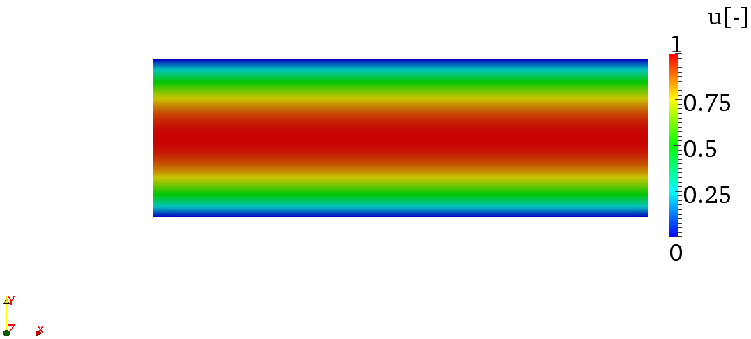
Figure 2.1: u-component of the velocity
$NEK/IncNavierStokesSolver). $NEK/IncNavierStokesSolver) executable encapsulates the nonlinear equations as well as
the stability tools. Therefore, when you setup either a nonlinear incompressible
problem or an incompressible stability problem you should use the same executable -
i.e.:$NEK/IncNavierStokesSolver file.xml.In the folder $NEKTUTORIAL/base you will find the file Channel-Base.xml which contains the
geometry along with the necessary parameters to solve the problem. The GEOMETRY section
defines the mesh of the problem and it is generated automatically as you have seen in the
previous task. The expansion type and order is specified in the EXPANSIONS section. An
expansion basis is applied to a geometry composite, where by composite we mean a collection
of mesh entities (specifically here, a collection of mesh elements), specified in the
GEOMETRY section. A default entry is always included by the $NEK/NekMesh utility. In
this case the composite C[0] refers to the set of all elements. The FIELDS attribute
specifies the fields for which this expansion should be used. The TYPE attribute
specifies the kind of the polynomial basis functions to be used in the expansion. For
example,
Note that all the results obtained in this tutorial refers to the expansion parameters just
defined (i.e. NUMMODES="11" FIELDS="u,v,p" TYPE="GLL_LAGRANGE").
In order to complete the problem definition and generate the base flow we need to specify a
section called CONDITIONS in the session file. If we examine Channel-Base.xml, we can see
how to define the conditions of the particular problem to solve.
In particular, the CONDITIONS section contains the following entries:
SOLVERINFO) such as the equation, the projection type (Continuous or
Discontinuous Galerkin), the evolution operator (Nonlinear for non-linear Navier-Stokes,
Direct1 ,
Adjoint or TransientGrowth for linearised forms) and the analysis driver to
use (Standard, Arpack or ModifiedArnoldi), along with other properties.
The solver properties are specified as quoted attributes and have the form
SOLVERINFO section of Channel-Base.xml:
Note: The bits to be completed are identified by …in this file.
EQTYPE to UnsteadyNavierStokes to select the unsteady incompressible
Navier-Stokes equations,
EvolutionOperator to Nonlinear in order to select the non-linear
Navier-Stokes,
Projection property to Continuous in order to select the continuous
Galerkin approach,
Driver to Standard in order to perform standard time-integration.PARAMETERS) are specified as name-value pairs:
Parameters may be used within other expressions, such as function definitions, boundary conditions or the definition of other subsequently defined parameters.
Re, that represents the Reynolds number, and
Kinvis, which represents the kinematic viscosity. Now set the Reynolds number to 7500
and the kinematic viscosity to 1∕Re - i.e.<P> Re = 7500 </P><P> Kinvis = 1/Re </P>VALUE entry which can be
an expression.
VARIABLES).
BOUNDARYREGIONS) in terms of composites
defined in the GEOMETRY section and the conditions applied on those boundaries
(BOUNDARYCONDITIONS). Boundary regions have the form
The boundary conditions enforced on a region take the following format and must
define the condition for each variable specified in the VARIABLES section to ensure the
problem is well-posed.
The REF attribute for a boundary condition region should correspond to the
ID="[INDEX]" of the desired boundary region specified in the BOUNDARYREGIONS
section.
FUNCTION), in terms of x, y,
z and t, such as initial conditions, forcing functions, and exact solutions. The VARIABLES
represent the components of the specific function in a specified direction and they must
be the same for every function.
Alternatively, one can specify the function using an external Nektar++ field file. For
example, this will be used to specify the InitialConditions or ExactConditions.
BodyForce):
fx = 2ν = 2*Kinvis.
CONDITIONS:
It is possible to specify an arbitrary initial condition. In this case, it was decided to start from the exact solution of the problem in order to have a steady state in just few iterations. If the initial condition is not specified, it will be set to zero by default.
This completes the specification of the problem.
Channel-Base.xml session file by
typing:
$NEK/IncNavierStokesSolver Channel-Base.xml
At the end of the simulation, the fields will be written to a binary file Channel-Base.fld and
the L2 error (using the given exact solution) and the L∞ error will be printed on the terminal
for each of the variables.
In particular, the terminal screen should look like this:
The final step regarding the base flow is to visualise the flow fields. Specifically, we need to
convert convert the .fld file into a format readable by a visualisation post-processing tool. In
this tutorial we decided to convert the .fld file into a VTK format and to use the open-source
visualisation package called Paraview .
$NEK/FieldConvert Channel-Base.xml Channel-Base.fld Channel-Base.vtu
Now open Paraview and use File ->Open, to select the VTK file, click the ’Apply’ button to render the geometry, and select each field in turn from the left-most drop-down menu on the toolbar to visualise the output.
Note: You can also open this type of file in VisIt.
In figure 2.1 we show how the base flow just computed should look like.
$NEK/FieldConvert Channel-Base.xml Channel-Base.fld Channel-Base.dat