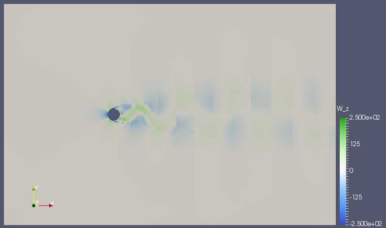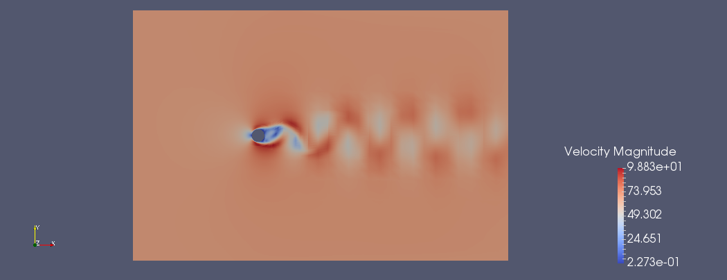
Figure 4.1: Instantaneous Velocity Flow Field
Now that the simulation has been completed, we need to post-process the file in order to visualise the results. In order to do so, we can use the built-in post-processing routines within Nektar + +. In particular we can use the following command:
$NEK/FieldConvert
CylinderSubsonic_NS.xml CylinderSubsonic_NS.fld CylinderSubsonic_NS.vtu.Which generates a .vtu file that is a readable format for the open-source package Paraview.
We can now open the .vtu file just generated and visualise it with Paraview. If we want to
monitor the evolution of the simulation we can make an animation in Paraview by converting
successive .chk files into .vtu
FinTime to 0.6 and run the simulation. In
order to do that, define the number of steps NumSteps as the ratio of the FinalTime to the
time-step TimeStep and set the FinalTime. Remember to use MPI in order to reduce the
simulation time.To create the animation we need to convert the .xml files into .vtu format. To avoid typing the same command several times, create a routine to create the different .vtu files. Once all the .vtu files are created (they are found in the completed folder), open them in paraview as a group (i.e File/Open and select all of them without expanding the tab).
If the final time is set to 0.6 and the .chk files are obtained every 400 steps. The animation created with the last 20 files should look like the CylinderSubsonic_NS.ogv video included in the completed folder.
Convert the .xml and .fld files into a .vtu format as shown in Task 4.1.
Calculate Vorticity
To perform the vorticity calculation and obtain an output data containing the vorticity solution, the user can run:
$NEK/FieldConvert -m vorticity CylinderSubsonic_NS.xml CylinderSubsonic_NS.fld
CylinderSubsonic_NS_vort.fld
Extract Wall Shear Stress
To obtain the wall shear stress vector and magnitude, the user can run:
FieldConvert -m wss:bnd=0:addnormals=0 CylinderSubsonic_NS.xml
CylinderSubsonic_NS.fld CylinderSubsonic_NS_wss.fld
The option bnd specifies which boundary region to extract. In this case the boundary region
ID of the cylinder is 0. If the addnormals is turned on, Nektar + + additionally outputs the
normal vector of the extracted boundary region.
In order to process the ouput file(s) you will need an .xml file of the same region. In order to do that we can use the NekMesh module extract:
NekMesh -m extract:surf=100 CylinderSubsonic_NS.xml bl.xml
Note, for NekMesh the surface ID we want to extract corresponds to the composite number of the cylinder surface -i.e 100.
To process the surface file one can use:
FieldConvert bl.xml CylinderSubsonic_NS_wss.fld
CylinderSubsonic_NS_wss.vtu
This command will generate a .dat file with the flow field information in the cylinder wall. It will produce the information of the density rho, the fluxes rhou, rhov and E, the pressure p, the sound velocity a, the Mach number Mach, the sensor values Sensor, the shear values Shearx, Sheary and Shearmag and the norms normx and normy for the different x and y coordinated along the cylinder. These files can be obtained from the completed folder.
This completes the tutorial.