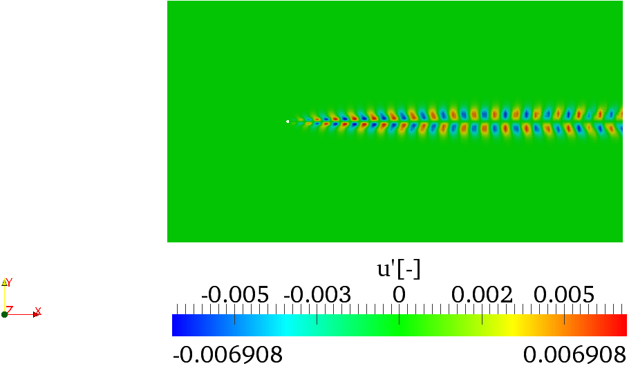
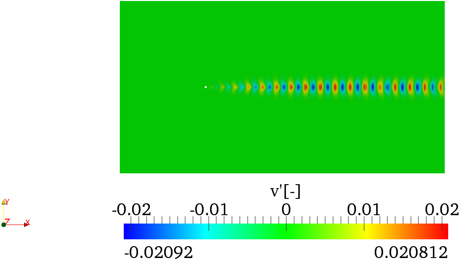
Figure 3.1: u′-component and v′-component of the eigenmode
In the folder $NEKTUTORIAL/stability/Direct there are the files that are required for the
direct stability analysis. Since, the computation would normally take several hours to
converge, we will use a restart file and a Krylov-space of just κ = 4. Therefore, it
will be possible to obtain the eigenvalue and the corresponding eigenmode after 2
iterations.
Cylinder_Direct.rst.The simulation should converge in 6 iterations and the terminal screen should look similar to the one below:
=======================================================================
                EquationType: UnsteadyNavierStokes
                Session Name: Cylinder_Direct
                Spatial Dim.: 2
          Max SEM Exp. Order: 7
              Expansion Dim.: 2
             Projection Type: Continuous Galerkin
                   Advection: explicit
                   Diffusion: explicit
                   Time Step: 0.0008
                No. of Steps: 1250
         Checkpoints (steps): 1000
            Integration Type: IMEXOrder2
=======================================================================
        Arnoldi solver type    : Arpack
        Arpack problem type    : LM
        Single Fourier mode    : false
        Beta set to Zero       : false
        Evolution operator     : Direct
        Krylov-space dimension : 4
        Number of vectors      : 2
        Max iterations         : 500
        Eigenvalue tolerance   : 1e-06
======================================================
Initial Conditions:
  - Field u: from file Cylinder_Direct.rst
  - Field v: from file Cylinder_Direct.rst
  - Field p: from file Cylinder_Direct.rst
Writing: "Cylinder_Direct_0.chk"
        Inital vector       : input file
Iteration 0, output: 0, ido=1 Writing: "Cylinder_Direct_1.chk"
Steps: 1250     Time: 1            CPU Time: 46.5477s
Time-integration  : 46.5477s
Writing: "Cylinder_Direct.fld"
Iteration 1, output: 0, ido=1 Writing: "Cylinder_Direct_1.chk"
Steps: 1250     Time: 2            CPU Time: 41.7221s
Time-integration  : 41.7221s
Iteration 2, output: 0, ido=1 Writing: "Cylinder_Direct_1.chk"
Steps: 1250     Time: 3            CPU Time: 41.8717s
Time-integration  : 41.8717s
Iteration 3, output: 0, ido=1 Writing: "Cylinder_Direct_1.chk"
Steps: 1250     Time: 4            CPU Time: 41.9465s
Time-integration  : 41.9465s
Iteration 4, output: 0, ido=1 Writing: "Cylinder_Direct_1.chk"
Steps: 1250     Time: 5            CPU Time: 41.987s
Time-integration  : 41.987s
Iteration 5, output: 0, ido=1
Writing: "Cylinder_Direct_1.chk"
Steps: 1250     Time: 6            CPU Time: 42.2642s
Time-integration  : 42.2642s
Iteration 6, output: 0, ido=99
Converged in 6 iterations
Converged Eigenvalues: 2
         Magnitude   Angle       Growth      Frequency
EV: 0 0.9792      0.726586    -0.0210196  0.726586
Writing: "Cylinder_Direct_eig_0.fld"
EV: 1 0.9792      -0.726586   -0.0210196  -0.726586
Writing: "Cylinder_Direct_eig_1.fld"
L 2 error (variable u) : 0.0501837
L inf error (variable u) : 0.0296123
L 2 error (variable v) : 0.0635524
L inf error (variable v) : 0.0355673
L 2 error (variable p) : 0.0344665
L inf error (variable p) : 0.0176009
After the direct stability analysis, it is now interesting to compute the eigenvalues and
eigenvectors of the adjoint operator A* that allows us to evaluate the effects of generic initial
conditions and forcing terms on the asymptotic behaviour of the solution of the
linearised equations. In the folder Cylinder/Stability/Adjoint there is the file
Cylinder_Adjoint.xml that is used for the adjoint analysis.
EvolutionOperator to Adjoint, the Krylov space to 4 and compute
the leading eigenvalue and eigenmode of the adjoint operator, using the restart file
Cylinder_Adjoint.rstThe solution should converge after 4 iterations and the terminal screen should look like this:
=======================================================================
                EquationType: UnsteadyNavierStokes
                Session Name: Cylinder_Adjoint
                Spatial Dim.: 2
          Max SEM Exp. Order: 7
              Expansion Dim.: 2
             Projection Type: Continuous Galerkin
                   Advection: explicit
                   Diffusion: explicit
                   Time Step: 0.001
                No. of Steps: 1000
         Checkpoints (steps): 1000
            Integration Type: IMEXOrder3
=======================================================================
        Arnoldi solver type    : Arpack
        Arpack problem type    : LM
        Single Fourier mode    : false
        Beta set to Zero       : false
        Evolution operator     : Adjoint
        Krylov-space dimension : 4
        Number of vectors      : 2
        Max iterations         : 500
        Eigenvalue tolerance   : 0.001
======================================================
Initial Conditions:
Field p not found.
  - Field u: from file Cylinder_Adjoint.rst
  - Field v: from file Cylinder_Adjoint.rst
  - Field p: from file Cylinder_Adjoint.rst
Writing: "Cylinder_Adjoint_0.chk"
        Inital vector       : input file
Iteration 0, output: 0, ido=1 Steps: 1000     Time: 27     CPU Time: 42.0192s
Writing: "Cylinder_Adjoint_1.chk"
Time-integration  : 42.0192s

Writing: "Cylinder_Adjoint.fld"
Iteration 1, output: 0, ido=1 Steps: 1000     Time: 28     CPU Time: 37.1084s
Writing: "Cylinder_Adjoint_1.chk"
Time-integration  : 37.1084s
Iteration 2, output: 0, ido=1 Steps: 1000     Time: 29     CPU Time: 37.4794s
Writing: "Cylinder_Adjoint_1.chk"
Time-integration  : 37.4794s
Iteration 3, output: 0, ido=1 Steps: 1000     Time: 30     CPU Time: 37.3142s
Writing: "Cylinder_Adjoint_1.chk"
Time-integration  : 37.3142s
Iteration 4, output: 0, ido=99
Converged in 4 iterations
Converged Eigenvalues: 2
         Magnitude   Angle       Growth      Frequency
EV: 0 0.980493    0.727526    -0.0197     0.727526
Writing: "Cylinder_Adjoint_eig_0.fld"
EV: 1 0.980493    -0.727526   -0.0197     -0.727526
Writing: "Cylinder_Adjoint_eig_1.fld"
L 2 error (variable u) : 0.434746
L inf error (variable u) : 0.156905
L 2 error (variable v) : 0.698425
L inf error (variable v) : 0.120624
L 2 error (variable p) : 0.216948
L inf error (variable p) : 0.0676028
Note that, in spatially developing flows, the eigenmodes of the direct stability operator tend to be located far downstream while the eigenmodes of the adjoint operator tend to be located upstream and near to the body, as can be seen in figures 3.2 and 3.3. From the profiles of the eigemodes, it can be deducted that the regions with the maximum receptivity for the momentum forcing and mass injection are near the wake of the cylinder, close to the upper and lower sides of the body surface, in accordance with results reported in the literature.