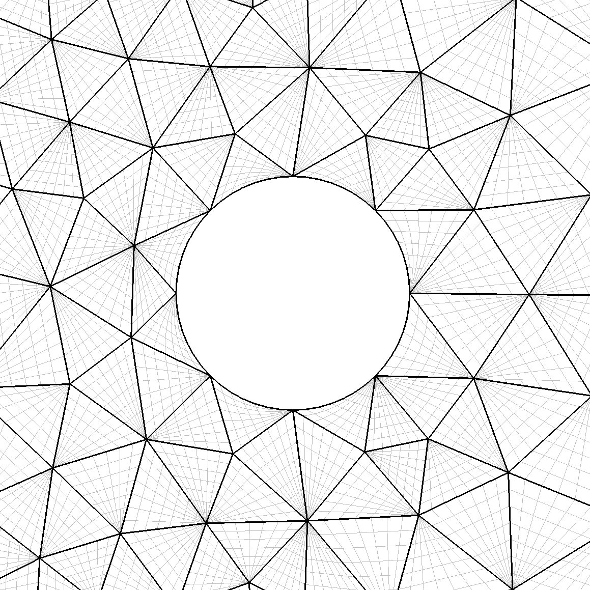
Figure 2.1: Initial triangular mesh generated by NekMesh and visualised in VisIt, using
8 subdivisions.
The mesh we make is for a simple 2D cylinder in a rectangular domain. We do this from a .stp file which has been provided.
$NEK/NekMesh cyl.mcf cyl.xml
More details about the generation process can be seen by enabling the verbose command line
option -v:
$NEK/NekMesh -v cyl.mcf cyl.xml
This will produce a Nektar++ mesh, which we now need to visualise.
$NEK/FieldConvert cyl.xml cyl.dat
or, for VTK output, for visualisation in ParaView or VisIt, run the command
$NEK/FieldConvert cyl.xml cyl.vtu
As these meshes are converted to a linear mesh, since this is what the visualisation software
supports, the curved elements can look quite faceted. To counteract this, we can add an
optional -nX command line option to FieldConvert, which increases the number of
subdivisions used to view the elements through interpolation.
$NEK/FieldConvert -n 8 cyl.xml cyl.vtu
and visualise the output, which should now look far smoother around the cylinder’s edge and give a better visualisation of the high-order elements.
The initial mesh can be seen in figure 2.1. Since we want to perform a simulation of flow over the cylinder, we now need to do some additional refinement, in order to produce a suitable mesh for our solvers. The first step is to change the configuration to generate a boundary layer mesh. To do this, we first change the mesh type in the configuration file to read
1 <I PROPERTY="MeshType" VALUE="2DBndLayer" />
In addition to this, we need to provide information to specify the boundary to be refined and the level of refinement required. This is done by adding four additional parameters to the configuration file:
1 <P PARAM="BndLayerSurfaces" VALUE="5,6,7,8" />
2 <P PARAM="BndLayerThickness" VALUE="0.25" />
3 <P PARAM="BndLayerLayers" VALUE="2" />
4 <P PARAM="BndLayerProgression" VALUE="1.5" />
This controls: the CAD surfaces (in this 2D case, the CAD curves), onto which the boundary layer will be added; the total thickness of the boundary layer; the number of layers in the boundary layer mesh; and the geometric progression used to define the reducing height of the boundary layer elements as they approach the surface.
cyl.mcf file, and change the mesh type to generate a boundary layer mesh using the
parameters above.We can now try to run some simulations on this mesh. A session file session_cyl.xml for the
cylinder mesh is provided, which will execute a low Reynolds number incompressible
simulation yielding classical vortex shedding. It is a relatively quick simulation and can run a
large number of convective lengths in a short time. But, using the mesh configuration
described above, the simulation will be quite under-resolved. You will notice that the vortices
will shed at a significant angle to the freestream.
$NEK/IncNavierStokesSolver cyl.xml session_cyl.xml
Process the final flow field visualisation with
$NEK/FieldConvert cyl.xml cyl.fld cyl.vtu
and visualise the results.
Flow around a cylinder is a canonical example of unsteady flow physics. It is possible to visualise the unsteady flow by getting the solver to write checkpoint files every certain number of timesteps. The output frequency is controlled by the parameter
1 <P> IO_CheckSteps = 50 </P>
$NEK/IncNavierStokesSolver cyl.xml session_cyl.xml
Finally, process these checkpoint files for visualisation by using the command
for i in {0..200}; do $NEK/FieldConvert cyl.xml cyl_${i}.chk cyl_${i}.vtu;
 done
Note that this is a bash command – if you use an alternative shell, such as tcsh, you may
need to alter this syntax. Load the files into your visualiser as a group, and use the frame
functions to view the flow as an unsteady animation.
The mesh which has been generated is very coarse and the simulation is lower order (P = 2), and as such the simulation is under-resolved. You should now be in a position to create a new mesh with your specifications and alter the simulation accordingly. You should note that increasing the resolution, you may affect the CFL condition and need to reduce the timestep.
A useful feature for this task is the ability to manually add refinement controls to
the mesh generation, which can be used to refine the wake of the cylinder so that
vortices can be captured accurately. This is done by adding a refinement tag to
the .mcf file, inside the MESHING XML tag, which for this example takes the form:
1<REFINEMENT>
2   <LINE>
3      <X1> -1.0 </X1>
4      <Y1> 0.0 </Y1>
5      <Z1> 0.0 </Z1>
6      <X2> 15.0 </X2>
7      <Y2> 0.0 </Y2>
8      <Z2> 0.0 </Z2>
9      <R> 1.5 </R>
10      <D> 0.4 </D>
11   </LINE>
12</REFINEMENT>
In this configuration, we define a line using two points, with coordinates (X1,Y1,Z1) and
(X2,Y2,Z2). R s the radius of influence of the refinement around this line, and D defines the size
of the elements within the refinement region.
If under your conditions the mesh has invalid elements you can also activate the variational
mesh generation tool, which will attempt to perform interior deformation by adding the
following tag inside the MESHING tag:
1   <BOOLPARAMETERS>
2      <P VALUE="VariationalOptimiser" />
3   </BOOLPARAMETERS>