Chapter 1
Introduction

This tutorial describes the use of the spectral/hp element framework Nektar++ to explore one of the classical and canonical problems of fluid dynamics: the Taylor-Green Vortex (TGV). Information on how to install the libraries, solvers, and utilities on your own computer is available on the webpage www.nektar.info.

The TGV flow case has analytical initial conditions and its exact solution is known from direct numerical simulation (DNS) using incompressible Navier-Stokes solvers. For this reason it is often used for code validation. Moreover, the TGV flow problem is a very instructive analysis case: through its numerical simulation, it is possible to study turbulent transition and decay, vortex dynamics and energy dissipation mechanisms ¹. In this tutorial we will focus on the solution of the TGV flow case in a 3D cube region within a time frame of 20 seconds, which is usually sufficient to observe the aforementioned phenomena. For now, we will restrict ourselves to a resolution of 64³ degrees of freedom using p = 8 order interpolants in a Continuous Galerkin (CG) projection. We will also have a look at the temporal evolution of the kinetic enery and its dissipation rate in the flow domain. The case with 128³ degrees of freedom is left as an optional exercise for the user.

The necessary files to complete this tutorial are included in the .zip folder downloaded using the link in Task 1.1. Under the folder tutorial, the user will find four subfolders, two for each resolution (64 or 128):

• Folder geometry64
  • TGV64_mesh.msh - Gmsh generated mesh data listing mesh vertices and elements for the 64³ case.

• Folder geometry128
  • TGV128_mesh.msh - Gmsh generated mesh data listing mesh vertices and elements for the 128³ case.

• Folder solver64
  • TGV64_mesh.xml - Nektar++ session file, generated with the $NEK/NekMesh utility, containing the 2D mesh for the 64³ case.
  • TGV64_conditions.xml - Nektar++ session file containing the solver settings for the 64³ case.
  • shell64.sh - A bash script with the required command structure to automatically run the simulation on the compute nodes at Imperial College London.

• Folder solver128
  • TGV128_mesh.xml - Nektar++ session file, generated with the $NEK/NekMesh utility, containing the 2D mesh for the 128³ case.
  • TGV128_conditions.xml - Nektar++ session file containing the solver settings for the 128³ case.
  • shell128.sh - A bash script with the required command structure to automatically run the simulation on the compute nodes at Imperial College London.

The folder completed that can also be found in the .zip contains the filled .xml files to be used as a check in case the user gets stuck, or to verify the correctness at the end of the tutorial.

Chapter 2
Background

The TGV is an exact solution of the incompressible Navier-Stokes equations:

+ V ⋅∇V	= -∇P + ν∇2V,
∇⋅V	= 0,

where V = (u,v,w) is the velocity of the fluid in the x, y and z directions respectively, P is the pressure, ρ is the density and ν is the kinematic viscosity. Note that the absence of a forcing function (body force) will result in viscosity dissipating all the energy in the fluid, which will then eventually come to rest.

In order to simulate the flow, the Velocity Correction Scheme will be used to evaluate the Navier-Stokes equations. This scheme uses a projection in which the velocity matrix and pressure are decoupled. For detailed information on the method, you can consult the User-Guide.

Quasi-3D Approach

Instead of constructing a 3D mesh of the domain and applying a spectral/hp discretisation in all three directions, it is more computationally efficient to use a quasi-3D approach. This approach allows the use of a spectral/hp expansion on a 2D mesh and to extend the computation in the third direction (typically the z-direction) using a simpler purely spectral harmonic discretisation (classically a Fourier expansion), if that direction is geometrically homogeneous. The user needs only specify the number of modes and basis type for the discretisation and the length along the z-direction.

Mesh and Boundary Conditions

The mesh we will use for the TGV flow is periodic in nature. It is therefore defined as -πL ≤ x,y,z ≤ πL, where L is the inverse of the wavenumber of the minimum frequency that can be captured on our mesh, i.e the largest length scale of our flow, known as the integral scale. It represents the size of the large, energy-carrying eddies responsible for most of the momentum transport. Given that the smallest length scale we can capture on our mesh Δx = _1D in one direction, it is clear that decreasing the integral scale L (for a periodic mesh, by decreasing its size) or increasing the number of mesh points N, allows us to capture smaller and smaller flow scales.

Since the TGV flow transitions to turbulence at a certain time, we would hope to capture the smallest turbulent length scales with our mesh. The smallest length scale η in one direction, as defined by Kolgomorov is:

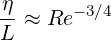(2.1)

Then the number of points required for a homogeneous mesh in 3D to capture the Kolgomorov scales is (with L = O(1)):

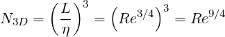(2.2)

Thus, for flow simulations of the TGV, which are usually run at Re = 1600, the number of uniform mesh points required to capture the smallest turbulent length scales is 16,190,861. The discretisation used in the current tutorial of N_3D = 64³ = 262,144 points does not have enough resolution to resolve these scales, and neither does the case with N_3D = 128³ = 2,097,152 points, left as an exercise. The case with N_3D = 256³ = 16,777,216 points would be sufficient but to simulate the flow with such a fine mesh requires the aid of a larger parallel computer, given the much larger memory requirements of the computation. When the flow is underresolved some stabilisation is typically required and this is why we will use a technique known as spectral vanishing viscosity for the lower resolution runs.

As mentioned above, the mesh used in this tutorial is a uniform square mesh of length -π ≤ x,y ≤ π (L = 1) containing 64 square elements, each with a spectral/hp expansion basis of order 8. This 2D mesh is then expanded in the z-direction to compute the quasi-3D flow. The homogeneous z-direction will be discretised using 64 planes. Boundary and initial conditions are also applied. The latter will be described in the following section. As for the former, given the periodic nature of the flow, periodic boundary conditions are applied on all edges of the mesh. The 2D meshes 64 and 128, showing all quadrature points, are shown in Fig. 2.1:

Initial Conditions

We are solving an initial value problem and in order to march the problem forward in time we need to prescribe initial conditions for all variables. For this case the initial conditions correspond to the TGV flow, given by:

u(x,y,z,t = 0)	= V 0 sin coscos,
v(x,y,z,t = 0)	= -V 0 cossin cos
w(x,y,z,t = 0)	= 0,
P(x,y,z,t = 0)	= 0.

The u and v velocity components of the vector field are shown in Fig 2.2. Note how these fields are formed by contiguous patches of velocity of same magnitude and opposed direction. The resulting flow, when both velocity fields are combined, is presented in Fig. 2.3 as vorticity contours. The vortical flow is formed by contiguous pairs of counter-rotating vortices, with strength Γ and -Γ.

Chapter 3
Configuring and Running the Solver

We will now proceed to set up the .xml file with the solver characteristics and parameters to run the simulation, using the case with 64³ as guidance. The settings for the 128³ are very similar, and it will be specified if otherwise.

The files required can be found under the folder $NEKTUTORIAL/solver64. The file TGV64_conditions.xml must be modified to set up the solver. Also in the same folder, TGV64_mesh.xml contains the definition of the mesh and the expansion bases that will be used for the computation.

The tag EXPANSIONS defines the type of polynomial expansions to be used on each element, and their order (NUMMODES= p + 1) as well as the FIELDS and COMPOSITES to which they are applied (in this case the whole domain C[0]).

The following sections all refer to modifications in the file TGV64_conditions.xml.

Parameters

The TGV case will be run at Re = 1600 with integral length scale L = 1 and initial velocity V ₀ = 1 so that the kinematic viscosity ν = 1∕1600. The temperature field is not included in the computations since it doesn’t influence the dynamics of the fluid. The physical time of the computation is based on the convective time scale t_c = L∕V ₀ = 1 and will be τ = 20t_c, with the first turbulent structures starting to build up at τ = 8t_c = 8.

These parameters apply for both 64³ and 128³. Remember to set the parameters following the typical XML syntax:

Note that expressions using a previously defined KEY can be inputted as a VALUE.

Once the flow parameters have been defined, we must define the discretisation in the homogeneous z-direction. Since we are interested in determining the flow on a cubic mesh, the length of the domain along the z-direction will also be L_z = 2π (not to be confused with the integral length scale, L). We must also specify the number of Fourier planes we are going to discretise our z-direction into. For a fully uniform mesh, we then choose N_z = 64 or 128, depending on the case that we are running. This corresponds to 32 or 64 complex Fourier modes, respectively.

Additionally, we also enable the spectral vanishing viscosity (SVV) feature which acts to dampen high-frequency oscillations in the solution which would otherwise introduce numerical instability.

These parameters also apply for both 64³ and 128³, except for N_z which must be set to 128 instead for the latter case. Note that π can be used directly with the keyword PI.

Solver Properties

We now declare how the flow will be solved. We will use the Velocity Correction Scheme (VCS) to solve the components of the unsteady Navier-Stokes equations separately, rather than as one single system. We must also specify the time integration method, which will be explicit-implicit of order 2, and the approach to be used when solving linear matrix systems of the form Ax = b that arise from the VCS scheme. Finally, we must describe how the homogeneous z-direction will be treated in the quasi 3D approach.

These properties apply for both 64³ and 128³ cases. Remember to set the property/value pairs following the typical XML syntax:

Boundary and Initial Conditions

The periodic boundary conditions for the domain are already defined for the user in the .xml file, under the tag BOUNDARYCONDITIONS. The initial conditions can be prescribed to the solver by means of a standard function.

Multi-variable functions such as initial conditions and analytic solutions may be specified for use in, or comparison with, simulations. These may be specified using expressions (<E>)

Filters

Turbulent flows, as is the TGV flow, have very high diffusivity. The random and chaotic motion of the fluid particles results in an increased momentum and mass convection as well as heat transfer, with the flow composed of fluid structures with a wide range of length scales. The large, energy-containing fluid structures inertially break down into smaller and smaller structures by vortex stretching, with an associated kinetic energy transfer between the scales. When these small fluid structures are of the size of the Kolgomorov length scales η, molecular viscosity becomes substantial and dissipates the kinetic energy into heat. As such, a good way of characterising turbulent flows is via the evolution of the kinetic energy or, more appropriately, via its dissipation rate.

Running the Solver

If you have not completed Task 1.2 or would like to test your configuration, the IncNavierStokesSolver can now be run with the XML files above to solve the TGV problem.

Chapter 4
Simulation Results

You will now have to post-process the files in order to see the results of the simulation. You may either use output files of your recent run or those provided in the folder completed/solver64. Amongst the output files, you can find the checkpoint files .chk and final file .fld that contain the state of the simulation at each time step; the modal energy file .mdl containing the energy spectrum of the Fourier modes; and the energy file .eny with the evolution of the kinetic energy and the enstrophy. Note that the folder completed/solver64 does not contain .chk files.

Both energy files are easily post-processed and can be converted to the MATLAB readable format .dat, just by changing the file extension. The checkpoint files however, must be converted to a standard visualisation data format so that they are readable with Paraview or other visualisation software.

The evolution of the kinetic energy of the flow is obtained by integrating the square of the velocity norm over the domain. Similarly, the enstrophy is calculated by integrating the square of the vorticity norm over the domain:

(4.1)

The enstrophy is a measure of the intensity of the vorticity and is related to dissipation effects of the flow. More precisely, under the assumption of incompressible flow, the enstrophy is related to the kinetic energy dissipation rate, ϵ, via the equation on the left. It is also defined as the rate of change of the kinetic energy, the equation on the right:

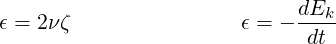(4.2)

Therefore, the dissipation rate can be calculated both from the enstrophy and numerically from the evolution of the kinetic energy. From the modal energy file, it is possible to evaluate the energy spectrum of the Fourier modes. This will in turn be helpful to identify what length scales carry the most energy. After post-processing the energy files on MATLAB, you should be able to produce the following figures, which depict the time evolution of the kinetic energy and enstrophy of the flow, as well as the evolution of the dissipation rate (both computed and enstrophy-based) and the energy spectrum:

Figure 4.1 Time evolution of the kinetic energy (left) and enstrophy (right).

Figure 4.2 Time evolution of numerically computed and enstrophy-based dissipation rates (left) and time evolution of the energy spectrum of the fourier modes (right).

The time evolution of the kinetic energy is well predicted by the spectral, quasi-3D computation. Since no force is applied to the fluid, the initial kinetic energy in the flow is progressively dissipated, with the dissipation rate peaking at around τ ≈ 9 when the turbulent fluid structures are formed. This is consistent with the enstrophy. The enstrophy, which is a measure of how vortical the flow is, peaks at the same time as the dissipation rate, τ ≈ 9: vortex stretching increases vorticity in the stretching direction and reduces the length scale of the fluid structures. Hence, when vorticity is at its highest, the flow is dominated by these small structures, which are responsible for the main viscous dissipation effects. The discrepancy between the numerically computed and enstrophy-based dissipation rates is directly related to the resolution of the mesh. The enstrophy-based dissipation rate being lower than the numerically calculated one means that, in the simulation, not all of the dissipation is due to the vorticity present in the flow. The low resolution of the mesh accentuates the numerical diffusion present in the spectral/hp element method and is the reason for the discrepancy.

Finally, from the evolution of the energy spectrum of the Fourier modes it is possible to infer how the flow behaves. Initially, all the energy is contained in the smallest wavenumbers, meaning that the flow is dominated by the large length scales. As time passes, the energy is progressively transferred to smaller and smaller scales (larger wavenumber). This energy in the small scales peaks between τ = 8 and τ = 10, when the flow is fully turbulent, and then dies out for all wavenumbers due to dissipation. This process is depicted in the figures below, through the z-component of the vorticity.

Advanced Task: 4.2 Running the simulation with a mesh of 128³ is a bit more computationally expensive and it is left as an optional exercise. If you do run this simulation, extract the information from the energy files and plot the time evolution of the kinetic energy, enstrophy and dissipation rate for both cases under the same graphs. Establish a qualitative and quantitave comparison between the results of using different resolutions to resolve the Taylor-Green Vortex flow.