Implement a short block of code where you see the comments “Write your code here”
which evaluates the loop
In this first exercise we will demonstrate how to integrate the function f(ξ) = ξ12 on the
standard segment ξ ∈ [−1,1] using Gaussian quadrature. The Gaussian quadrature weights
and zeros are coded in the LIbUtilities library and for future reference this can be found
under the directory $NEKDIST/library/LibUtilities/Foundations/. For the following
exercises we will access the zero and points from the PointsManager. The PointsManager is a
type of map (or manager) which requires a key defining known Gaussian quadrature types
called PointsKey.
In the $NEKDIST/tutorial/fundamentals-integration/tutorial directory open the file
named StdIntegration1D.cpp. Look over the comments supplied in the file which outline
how to define the number of quadrature points to apply, the type of Gaussian quadrature and
some arrays to hold the zeros, weights and solution. Finally a PointsKey is defined which
is then used to obtain the zeros and weights in two arrays called quadZeros and
quadWeights.
Implement a short block of code where you see the comments “Write your code here”
which evaluates the loop
To compile your code type
make StdIntegation1D
in the tutorial directory. When your code compiles successfully1 then type
./StdIntegration1D
You should now get some output similar to
We can also use Gauss-Lobatto-Legendre type integration rather than Gauss-Legendre type in the previous exercises. To do this we replace
with
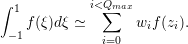
A straightforward extension of the one-dimensional Gaussian rule is to the two-dimensional standard quadrilateral region and similarly to the three-dimensional hexahedral region. Integration over Q2 = {−1 ≤ ξ1,ξ2 ≤ 1} is mathematically defined as two one-dimensional integrals of the form
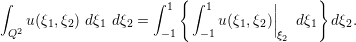
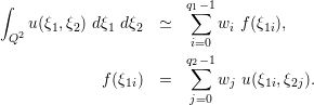
So if we replace the right-hand-side integrals with our one-dimensional Gaussian integration rules we obtain
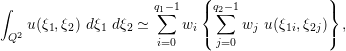
where q1 and q2 are the number of quadrature points in the ξ1 and ξ2 directions. This expression will be exact if u(ξ1,ξ2) is a polynomial and q1,q2 are chosen appropriately. To numerically evaluate this expression the summation over ‘i’ must be performed q1 times at every ξ2i point, that is,
Using a series of one-dimensional Gaussian quadrature rules as outlined above evaluate the
integral by completing the first part of the code in the file StdIntegration2D.cpp in the
directory
$NekDist/tutorial/fundamentals-integration/tutorial.
The quadrature weights and zeros in each of the coordinate directions have already been setup and are initially set to q1 = 6,q2 = 7 using a Gauss-Lobatto-Legendre quadrature rule. Complete the code by writing a structure of loops which implement the two-dimensional Gaussian quadrature rule2 . The expected output is given below). Also verify that the error is zero when q1 = 8,q2 = 9.
Recall that to compile the file you type
make StdIntegration2D
When executing the tutorial with the quadrature order q1 = 6,q2 = 7 you should get an output of the form:
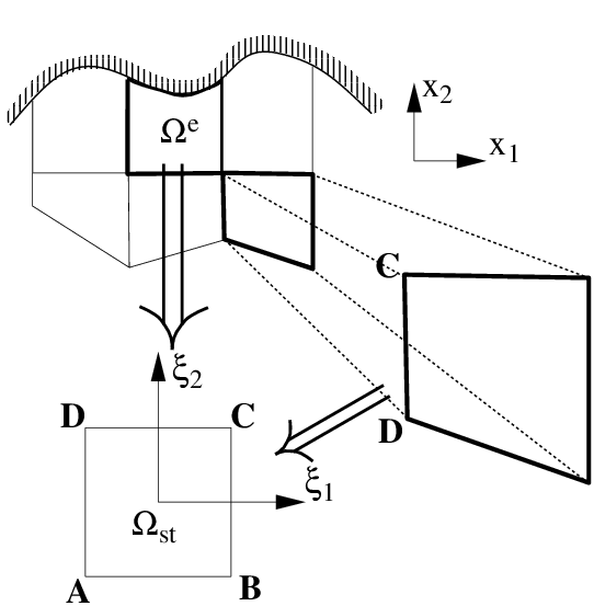
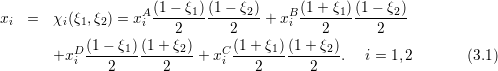
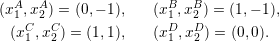
For elemental shapes with straight sides a simple mapping may be constructed using a linear mapping similar to the vertex modes of a hierarchical/modal expansion. For the straight-sided quadrilateral with vertices labeled as shown in figure 3.1(b) the mapping can be defined as:
If we denote an arbitrary quadrilateral region by Ωe which is a function of the global Cartesian coordinate system (x1,x2) in two-dimensions. To integrate over Ωe we transform this region into the standard region Ωst defined in terms of (ξ1,ξ2) and we have

where J2D is the two-dimensional Jacobian due to the transformation, defined as:
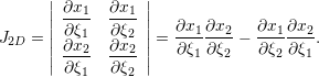 | (3.2) |
As we have assumed that we know the form of the mapping [i.e., x1 = χ1(ξ1,ξ2), x2 = χ2(ξ1,ξ2)] we can evaluate all the partial derivatives required to determine the Jacobian. If the elemental region is straight-sided then we have seen that a mapping from (x1,x2) → (ξ1,ξ2) is given by equations (3.1).
This is clearly similar to the previous exercise. However, as we are calculating the integral of a function defined on a local element rather than on a reference element, we have to take into account the geometry of the element. Therefore, the implementation is altered in two ways:
In the file LocIntegration2D.cpp you are provided with the same set up as the previous task
but now with a definition of the coordinate mapping included. Evaluate the expression for the
Jacobian analytically. Then write a line of code in the loop for the Jacobian as indicated by
the comments “Write your code here”. When you have written your expression you can
compile the code with the command
make LocIntegration2D
Verify that the error is not equal to zero when q1 = 8,q2 = 9. Why might this be the case?3 .
Using the quadrature order specified in the file your output should look like: