+ u ⋅∇u
 + u ⋅∇T
This tutorial provides an overview of utilising the spectral/hp element framework Nektar++ for the numerical solution of a classical fluid dynamics problem: Rayleigh–Bénard Convection (RBC). The tutorial will delve into the direct numerical simulation and linear stability analysis of a two-dimensional RBC.
Information on how to install the libraries, solvers, and utilities on your own computer is available on the webpage www.nektar.info. This tutorial assumes the reader has already completed the previous tutorial in the Flow Stability series on the channel and already has the necessary software installed.
Downloaded the tutorial files: rbc.tar.gz
Unpack it using unzip rbc.tar.gz to produce a directory rbc with subdirectories
called tutorial and complete. We will refer to the tutorial directory as
$NEKTUTORIAL.
The dynamical equations that describe Rayleigh–Bénard Convection (RBC) under Boussinesq approximation in the non-dimensional form are
| + u ⋅∇u | = -∇p + RaPrTey + Pr∇2u, | (1.1) |
| + u ⋅∇T | = ∇2T, | (1.2) |
| ∇⋅u | = 0, | (1.3) |
where u and T are the velocity and temperature fields, respectively, and ey is the buoyancy direction. Here p is the modified pressure including the buoyancy term accounting for the reference temperature. Flow is controlled by two non-dimensional numbers, the Rayleigh number Ra and the Prandtl number Pr.
By decomposing the velocity, temperature and pressure in the equations (1.2-1.3) as a summation of a base flow (U,,P) and perturbation (u′,T′,p′), such that
| u | = U + u′ | (1.4) |
| T | = + T′ | (1.5) |
| p | = P + p′, | (1.6) |
and retaining first-order terms only yields the linearised equations governing the evolution of infinitesimal perturbations:
 + u′⋅∇U + (U ⋅∇)u′ + u′⋅∇U + (U ⋅∇)u′ | = -∇p′ + RaPrT′e y + Pr∇2u′, | (1.7) |
 + u′⋅∇ + U ⋅∇T′ + u′⋅∇ + U ⋅∇T′ | = ∇2T′, | (1.8) |
| ∇⋅u′ | = 0. | (1.9) |
In Chapter 2, we will validate a case of two-dimensional RBC in a domain of aspect
ratio 2.02. In Chapter 3, we will discuss the linear stability analysis for a no-slip
boundary condition at top and bottom plates, and will estimate the critical value of
Rayleigh number. The files contained in the $NEKTUTORIAL directory are as follows:
Folder geometry
rbc.geo - Gmsh file that contains the geometry of the problem.
rbc.msh - Gmsh generated mesh data listing mesh vertices and elements.
Folder DNS/Ra_5e3_Pr_0p71
rbc-DNS.xml - Nektar++ session file, generated with the $NEK/NekMesh
utility, for computing the flow for Ra = 5000 and Pr = 0.71.
Folder LSA/Ra_1900
rbc-LSA.xml - Nektar++ session file, generated with $NEK/NekMesh for the
linear stability analysis for Ra = 1900 and Pr = 0.71.
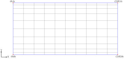
The first step is to generate a mesh that is readable by Nektar++. The files necessary in this
section can be found in $NEKTUTORIAL/geometry/. To achieve this task, we use Gmsh in
conjunction with the Nektar++ pre-processing utility called $NEK/NekMesh. Specifically, we
first generate the mesh in figure 1.1 using Gmsh and successively, we convert it into a suitable
Nektar++ format using $NEK/NekMesh. For all calculations in this tutorial, we fix Lx = 2.02
and Ly = 1.0 to maintain the aspect ratio of 2.02.
rbc.msh can be generated using Gmsh by running the following command:
gmsh -2 rbc.geo
rbc.xml can be generated using the module peralign available with the
pre-processing tool $NEK/NekMesh:
$NEK/NekMesh -m peralign:surf1=2:surf2=3:dir=x rbc.mesh rbc.xml
where surf1 and surf2 correspond to the periodic physical surface IDs specified in
Gmsh (in our case the inflow has a physical ID=2 while the outflow has a physical
ID=3) and dir is the periodicity direction (i.e. the direction normal to the inflow
and outflow boundaries - in our case x).