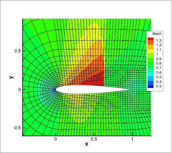
Compressible flow is characterised by abrupt changes in density within the flow domain often referred to as shocks. These discontinuities lead to numerical instabilities (Gibbs phenomena). This problem is prevented by locally adding a diffusion term to the equations to damp the numerical fluctuations. These fluctuations in an element are identified using a sensor algorithm which quantifies the smoothness of the solution within an element. The value of the sensor in an element is defined as
|
| (9.8) |
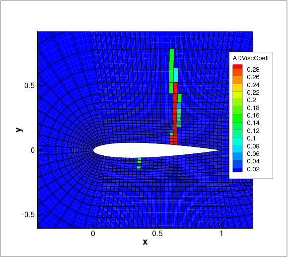
An artificial diffusion term is introduced locally to the Euler equations to deal with flow discontinuity and the consequential numerical oscillations. Two models are implemented, a non-smooth and a smooth artificial viscosity model.
For the non-smooth artificial viscosity model the added artificial viscosity is constant in each element and discontinuous between the elements. The Euler system is augmented by an added laplacian term on right hand side of equation 9.1. The diffusivity of the system is controlled by a variable viscosity coefficient ϵ. The value of ϵ is dependent on ϵ0, which is the maximum viscosity that is dependent on the polynomial order (p), the mesh size (h) and the maximum wave speed and the local sensor value. Based on pre-defined sensor threshold values, the variable viscosity is set accordingly
 | (9.9) |
For the smooth artificial viscosity model an extra PDE for the artificial viscosity is appended to the Euler system
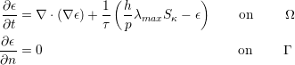 | (9.10) |
where Sκ is a normalised sensor value and serves as a forcing term for the artificial viscosity. A
smooth artificial viscosity distribution is obtained.
To enable the smooth viscosity model, the following line has to be added to the SOLVERINFO
section:
Furthermore, the extra viscosity variable eps has to be added to the variable list:
A similar addition has to be made for the boundary conditions and initial conditions. The tests that have been run started with a uniform homogeneous boundary condition and initial condition. The following parameters can be set in the xml session file:
where for now FH and FL are used to tune which range of the sensor is used as a
forcing term and C1 and C2 are fixed constants which can be played around with
to make the model more diffusive or not. However these constants are generally
fixed.
A sensor based p-adaptive algorithm is implemented to optimise the computational cost and
accuracy. The DG scheme allows one to use different polynomial orders since the fluxes over
the elements are determined using a Riemann solver and there is now further coupling
between the elements. Furthermore, the initial p-adaptive algorithm uses the same
sensor as the shock capturing algorithm to identify the smoothness of the local
solution so it rather straightforward to implement both algorithms at the same
time.
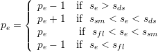
The polynomial order in each element can be adjusted based on the sensor value that is
obtained. Initially, a converged solution is obtained after which the sensor in each element is
calculated. Based on the determined sensor value and the pre-defined sensor thresholds, it is
decided to increase, decrease or maintain the degree of the polynomial approximation in each
element and a new converged solution is obtained.
 | (9.11) |
For now, the threshold values se, sds, ssm and sfl are determined empirically by looking at the sensor distribution in the domain. Once these values are set, two .txt files are outputted, one that has the composites called VariablePComposites.txt and one with the expansions called VariablePExpansions.txt. These values have to copied into a new .xml file to create the adapted mesh.