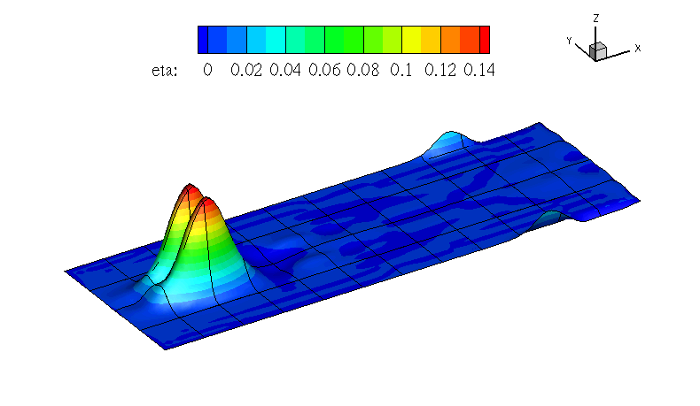
This example, provided in RossbyModon_Nonlinear_DG.xml is of a discontinuous Galerkin
simulation of the westward propagation of an equatorial Rossby modon.
For what concern the ShallowWaterSolver the <SOLVERINFO> section allows us to specify the
solver, the type of projection (continuous or discontinuous), the explicit time integration
scheme to use and (in the case the discontinuous Galerkin method is used) the choice of
numerical flux. A typical example would be:
In the <PARAMETERS> section we, in addition to the normal setting of time step etc., also define
the acceleration of gravity by setting the parameter "Gravity":
We specify f which is the Coriolis parameter and d denoting the still water depth as analytic functions:
Initial values and boundary conditions are given in terms of primitive variables (please note
that also the output files are given in terms of primitive variables). For the discontinuous
Galerkin we typically enforce any slip wall boundaries weakly using symmetry technique. This
is given by the USERDEFINEDTYPE="Wall" choice in the <BOUNDARYCONDITIONS> section:
After the input file has been copied to the build directory of the ShallowWaterSolver the
code can be executed by:
After the final time step the solver will write an output file RossbyModon_Nonlinear_DG.fld.
We can convert it to tecplot format by using the FieldConvert utility. Thus we execute the
following command:
This will generate a file called RossbyModon_Nonlinear_DG.dat that can be loaded directly
into tecplot: