2.2 The Structure of Nektar++
When we speak of Nektar++, it often means different things to different people, all under an
umbrella of code. For the founders of Nektar++, the view was that the core of Nektar++ was
the library, and that everything else was to be built around or on top of our basic
spectral/hp framework. For others, the heart of Nektar++ are its solvers – the collection
of simulation codes, built upon the library, that enable users to solve science and
engineering problems. For a smaller group of people, it is all the add-ons that we provide
in our utilities, from our mesh generation techniques to our visualization software
ideas.
For the purposes of this document, we will structure our discussions into three main parts:
library functionality, solvers and utilities. In this section, we will provide an overview of the
structure of the libraries. We will start by giving a quick overview of the basic subdirectories
contained within library and their purpose. We will then provide a bottom-up description of
how the library can be viewed, as well as a top-down perspective. Each perspective
(bottom-up or top-down) is fully consistent with each other; the advantage of these
approaches is that they help the future developer understand the library as someone trying to
build up towards our solvers, or conversely someone trying to understand our solver
functionality having already been a solver user and now trying to understand the library
components on which it was built.
The basic subdirectories with the library are as follows:
LibUtilities: This library contains all the basic mathematical and computer science building
blocks of the Nektar++ code.
StdRegions: This library contains the objects that express “standard region” data and
operations. In one dimension, this is the StdSegment. In two dimensions, this is the StdTri
(Triangle) and StdQuad (Quadrilateral). In three dimensions, this is the StdTet (Tetrahedra),
StdHex (Hexahedra), StdPrism (Prism) and StdPyr (Pyramid). These represent the seven
different standardized reference regions over which we support differentiation and
integration.
SpatialDomains: This library contains the mesh and elemental geometric information. In
particular, this part of the library deals with the basic mesh data structures, and the mapping
information (such as Jacobians) from StdRegions to LocalRegions.
LocalRegions: This library contains objects that express data and operations on
individual physical elements of the computational mesh. Local regions are spectral/hp
elements in world-space (either straight-/planar-sided or curved-sided). Using C++
terminology, a local region object is-a standard region object and has-a spatial domain
object.
MultiRegions: This library holds the data structures that represent sets of elements (local
regions). At the most fundamental level, these represent the union of local regions into a
(geometrically-contiguous) space. By specifying the interaction of these elements, the function
space they represent and/or the approximation method is defined. It is at this point in the
hierarchy that a set of (local region) elements can be thought of as representing a dG or cG
field.
Collections: In this library we amalgamate, in a linear algebra sense, the action of key
operators on multiple (standard region or local region) elements into a single, memory-efficient
block. These strategies depend on external factors such as BLAS implementation and the
geometry of interest.
GlobalMapping: This library supports the analytical mapping of complex physical domains
to simpler computational domains.
NekMeshUtils: This library contains processing modules for the generation (potentially from
CAD geometries), conversion and manipulation of high-order meshes.
SolverUtils: This library contains data structures and algorithms which form the basis of
solvers, or provide auxiliary functionality.
UnitTests: This part of the library contains unit tests that allow us to verify the correctness
of the core functionality within Nektar++. These are useful for verifying that new additions or
modifications to the lower-levels of the code do not compromise existing functionality or
correctness.
Bottom-Up Perspective
The bottom-up perspective on the library is best understood from Figures 2.1 – 2.2. In Figure
2.1, we take the view of understanding the geometric regions over which we build
approximations. Our starting point is within the StdRegions library, in which we define our
canonical standard regions. There are seven fundamental regions supported by Nektar++:
segments (1D), triangles and quadrilaterals (2D) and tetrahedra, hexahedra, prisms and
pyramids (3D). Since we principally employ Gaussian quadrature, these regions are defined
by various tensor-product and collapsing of the compact interval [-1,1]. For the
purposes of illustration, let us use a quadrilateral as our example. The StdQuadExp is a
region defined on [-1,1] × [-1,1] over which we can build approximations ϕe(ξ1,ξ2).
Typically ϕe is based upon polynomials in each coordinate direction; using linear
functions in both directions yields the traditional Q(1) space in traditional finite
elements.
Since ϕe(ξ1,ξ2) lives on Q = [-1,1] × [-1,1] (i.e. ϕe : Q→ ℝ) and is for this example
polynomial, we can integrate it exactly (to machine precision) using Gaussian integration, and
we can differentiate it by writing it in a Lagrange basis and forming a differential operator
matrix to act on values of the function evaluated at points. If the function were not
polynomial but instead only a smooth function, we could approximate it with quadrature and
decide an appropriate basis by which to approximate its derivatives. All the routines needed
for differentiating and integrating polynomials over various standard regions are contained
within the StdRegions directory (and will be discussed in Chapter 5). A local region
expansion, such as a basis defined on a quadrilateral element, QuadExp, is a linear
combination of basis functions over its corresponding standard region as mapped
by information contained within its spatial domain mapping. Local region class
definitions are in the LocalRegions directory (and will be discussed in Chapter 7). Using
the inheritance language of C++, we would say that a local region is-a standard
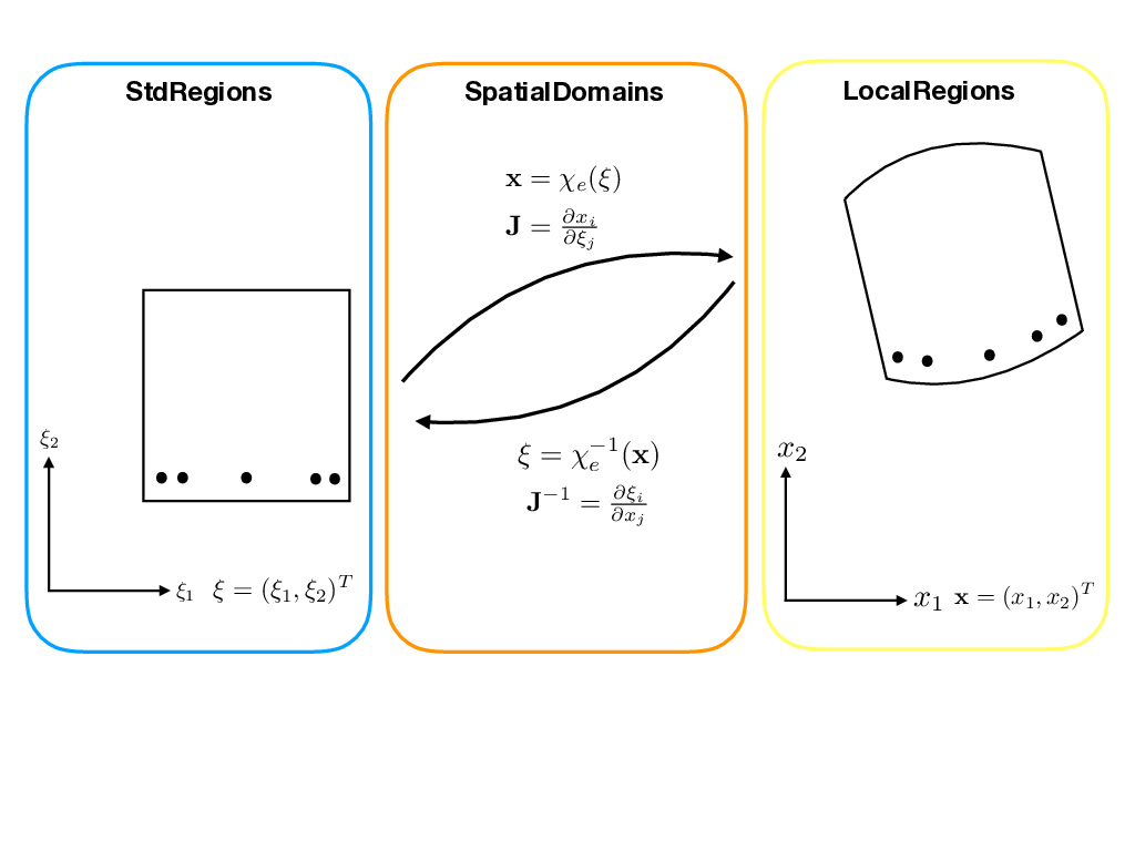
region and has-a spatial domain object. The SpatialDomains directory contains
information that expresses the mapping function χe(⋅) from the standard region to a local
region. SpatialDomains is explored in Chapter 6. In the case of our quad example, the
SpatialDomain object held by a QuadExp would connect the local region to its
StdRegion parent, and correspondingly would allow integration and differentiation
in world space (i.e., the natural coordinates in which the local expansion lives).
If E denotes our geometric region in world space and if F : E → ℝ is built upon
polynomials over its standard region, then we obtain F(x1,x2) = ϕe(χe-1(x1,x2)). Note
that even though ϕe is polynomial and χe is polynomial, the composition using the
inverse of χe is not guaranteed to be polynomial: it is only guaranteed to be a smooth
function.
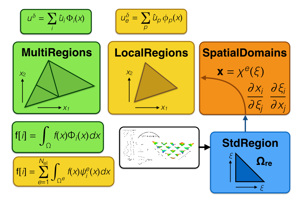
Putting this in the context of MultiRegions, we arrive at Figure 2.2. The MultiRegions
directory (which will be discussed in Chapter 9) contains various data structures that combine
local regions. One can think of a multi-region as being a set of local region objects in which
some collection of geometric and/or function properties are enforced. Conceptually, one can
have a set of local region objects that have no relationship to each other in space. This is a set
in the mathematical sense, but not really meaningful to us for solving approximation
properties. Most often we want to think of sets of local regions as being collections of elements
that are geometrically contiguous – that is, given any two elements in the set, we expect that
there exists a path that allows us to trace from one element to the next. Assuming a
geometrically continuous collection of elements, we can now ask if the functions built over
those elements form a piece-wise discontinuous approximation of a function over our
Multiregion or a piece-wise continuous C0 approximation of a function over our
Multiregion.
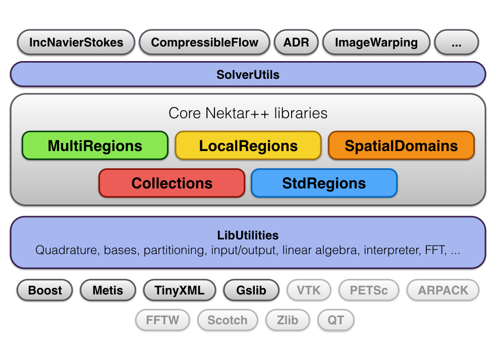
Top-Down Perspective
The top-down perspective on the library is best understood from Figure 2.3. From this
perspective, we are interested in understanding Nektar++ from the solvers various people have
contributed.