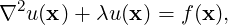
Most of the solvers in Nektar++, including the incompressible Navier-Stokes equations, rely on the solution of a Helmholtz equation,
|
| (9.1) |
an elliptic boundary value problem, at every time-step, where u is defined on a domain Ω of Nel non-overlapping elements. In this section, we outline the preconditioners which are implemented in Nektar++. Whilst some of the preconditioners are generic, many are especially designed for the modified basis only.
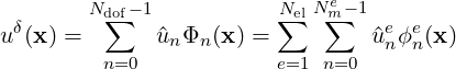
The standard spectral/hp approach to discretise (9.1) starts with an expansion in terms of the elemental modes:
 | (9.2) |
where Nel is the number of elements, Nme is the number of local expansion modes within the element Ωe, ϕne(x) is the nth local expansion mode within the element Ωe, ûne is the nth local expansion coefficient within the element Ωe. Approximating our solution by (9.2), we adopt a Galerkin discretisation of equation (9.1) where for an appropriate test space V δ we find an approximate solution uδ ∈ V δ such that

This can be formulated in matrix terms as

where H represents the Helmholtz matrix,  are the unknown global coefficients and f the
inner product the expansion basis with the forcing function.
are the unknown global coefficients and f the
inner product the expansion basis with the forcing function.
We first consider the C0 (i.e. continuous Galerkin) formulation. The spectral/hp expansion basis is obtained by considering interior modes, which have support in the interior of the element, separately from boundary modes which are non-zero on the boundary of the element. We align the boundary modes across the interface of the elements to obtain a continuous global solution. The boundary modes can be further decomposed into vertex, edge and face modes, defined as follows:
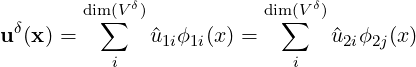
When the discretisation is continuous, this strong coupling between vertices, edges and faces leads to a matrix of high condition number κ. Our aim is to reduce this condition number by applying specialised preconditioners. Utilising the above mentioned decomposition, we can write the matrix equation as:
![[ ] [ ] [ ]
Hbb Hbi ^ub = ^fb
Hib Hii ^ui ^fi](developer-guide144x.png)
where the subscripts b and i denote the boundary and interior degrees of freedom respectively. This system then can be statically condensed allowing us to solve for the boundary and interior degrees of freedom in a decoupled manor. The statically condensed matrix is given by
![[ ] [ ] [ ]
Hbb - HbiH -1Hib 0 ^ub ^fb - HbiH -1^fi
H ii H ^u = ^ ii
ib ii i fi](developer-guide145x.png)
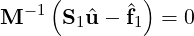
This is highly advantageous since by definition of our interior expansion this vanishes on the boundary, and so Hii is block diagonal and thus can be easily inverted. The above sub-structuring has reduced our problem to solving the boundary problem:

where S1 = Hbb -HbiHii-1Hib and  1 =
1 =  b -HbiHii-1
 i. Although this new system typically
has better convergence properties (i.e lower κ), the system is still ill-conditioned, leading to a
convergence rate of the conjugate gradient (CG) routine that is prohibitively slow. For this
reason we need to precondition S1. To do this we solve an equivalent system of the
form:
i. Although this new system typically
has better convergence properties (i.e lower κ), the system is still ill-conditioned, leading to a
convergence rate of the conjugate gradient (CG) routine that is prohibitively slow. For this
reason we need to precondition S1. To do this we solve an equivalent system of the
form:
where the preconditioning matrix M is such that κ is less than κ
 and
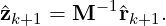
speeds up the convergence rate. Within the conjugate gradient routine the same
preconditioner M is applied to the residual vector
and
speeds up the convergence rate. Within the conjugate gradient routine the same
preconditioner M is applied to the residual vector  k+1 of the CG routine every
iteration:
k+1 of the CG routine every
iteration:
When utilising a hybridizable discontinuous Galerkin formulation, we perform a static condensation approach but in a discontinuous framework, which for brevity we omit here. However, we still obtain a matrix equation of the form

where Λ represents an operator which projects the solution of each face back onto the
three-dimensional element or edge onto the two-dimensional element. In this setting then,  consists of degrees of freedom for each egde (in 2D) or face (in 3D). The overall system does
not, therefore, results in a weaker coupling between degrees of freedom, but at the expense of
a larger matrix system.
consists of degrees of freedom for each egde (in 2D) or face (in 3D). The overall system does
not, therefore, results in a weaker coupling between degrees of freedom, but at the expense of
a larger matrix system.
Within the Nektar++ framework a number of preconditioners are available to speed up the convergence rate of the conjugate gradient routine. The table below summarises each method, the dimensions of elements which are supported, and also the discretisation type support which can either be continuous (CG) or discontinuous (hybridizable DG).
| Name | Dimensions | Discretisations |
Null | All | All |
Diagonal | All | All |
FullLinearSpace | 2/3D | CG |
LowEnergyBlock | 3D | CG |
Block | 2/3D | All |
FullLinearSpaceWithDiagonal | All | CG |
FullLinearSpaceWithLowEnergyBlock | 2/3D | CG |
FullLinearSpaceWithBlock | 2/3D | CG |
The default is the Diagonal preconditioner. The above preconditioners are specified through
the Preconditioner option of the SOLVERINFO section in the session file. For example, to
enable FullLinearSpace one can use:
Alternatively one can have more control over different preconditioners for each solution field
by using the GlobalSysSoln section. For more details, consult the user guide. The following
sections specify the details for each method.
Diagonal (or Jacobi) preconditioning is amongst the simplest preconditioning strategies. In this scheme one takes the global matrix H = (hij) and computes the diagonal terms hii. The preconditioner is then formed as a diagonal matrix M-1 = (hii-1).
The linear space (or coarse space) of the matrix system is that containing degrees of freedom corresponding only to the vertex modes in the high-order system. Preconditioning of this space is achieved by forming the matrix corresponding to the coarse space and inverting it, so that
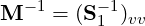
Since the mesh associated with higher order methods is relatively coarse compared with traditional finite element discretisations, the linear space can usually be directly inverted without memory issues. However such a methodology can be prohibitive on large parallel systems, due to a bottleneck in communication.
In Nektar++ the inversion of the linear space present is handled using the XXT library. XXT
is a parallel direct solver for problems of the form A =
=  based around a sparse factorisation
of the inverse of A. To precondition utilising this methodology the linear sub-space is gathered
from the expansion and the preconditioned residual within the CG routine is determined by
solving
based around a sparse factorisation
of the inverse of A. To precondition utilising this methodology the linear sub-space is gathered
from the expansion and the preconditioned residual within the CG routine is determined by
solving
The preconditioned residual  is then scattered back to the respective location in the global
degrees of freedom.
is then scattered back to the respective location in the global
degrees of freedom.
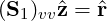
Block preconditioning of the C0 continuous system is defined by the following:
where diag[(S1)vv] is the diagonal of the vertex modes, (S1)eb and (S1)fb are block diagonal matrices corresponding to coupling of an edge (or face) with itself i.e ignoring the coupling to other edges and faces. This preconditioner is best suited for two dimensional problems.
In the HDG system, we take the block corresponding to each face and invert it. Each of these inverse blocks then forms one of the diagonal components of the block matrix M-1.
Low energy basis preconditioning follows the methodology proposed by Sherwin & Casarin. In this method a new basis is numerically constructed from the original basis which allows the Schur complement matrix to be preconditioned using a block preconditioner. The method is outlined briefly in the following.
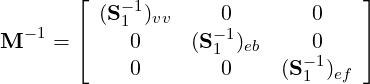
Elementally the local approximation uδ can be expressed as different expansions lying in the same discrete space V δ
Since both expansions lie in the same space it’s possible to express one basis in terms of the other via a transformation, i.e.

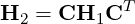
Applying this to the Helmholtz operator it is possible to show that,
For sub-structured matrices (S) the transformation matrix (C) becomes:
![[ R 0 ]
C =
0 I](developer-guide166x.png)
Hence the transformation in terms of the Schur complement matrices is:
Typically the choice of expansion basis ϕ1 can lead to a Helmholtz matrix that has undesirable properties i.e poor condition number. By choosing a suitable transformation matrix C it is possible to construct a new basis, numerically, that is amenable to block diagonal preconditioning.
![⌊ Svv Sve Svf ⌋ [ ]
| ST S S | Svv Sv,ef
S1 = ⌈ veT eTe ef ⌉ = STv,ef Sef,ef
S vf S ef Sff](developer-guide168x.png)
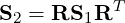
Applying the transformation S2 = RS1RT leads to the following matrix
![[ S + R ST + S RT + R S RT [S + R S ]AT ]
S2 = vv v v,efT v,ef v T v ef,ef v v,ef v ef,eTf
A[Sv,ef + Sef,efR v ] ASef,efA](developer-guide169x.png)
where ASef,efAT is given by
![[ T T T ]
ASef,efAT = See + Ref Sef + SefR ef + RefSffR ef Sef + RefSff
STef + Sff RTef Sff](developer-guide170x.png)
To orthogonalise the vertex-edge and vertex-face modes, it can be seen from the above that
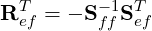
and for the edge-face modes:
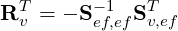
Here it is important to consider the form of the expansion basis since the presence of Sff-1 will lead to a new basis which has support on all other faces; this is problematic when creating a C0 continuous global basis. To circumvent this problem when forming the new basis, the decoupling is only performed between a specific edge and the two adjacent faces in a symmetric standard region. Since the decoupling is performed in a rotationally symmetric standard region the basis does not take into account the Jacobian mapping between the local element and global coordinates, hence the final expansion will not be completely orthogonal.
The low energy basis creates a Schur complement matrix that although it is not completely orthogonal can be spectrally approximated by its block diagonal contribution. The final form of the preconditioner is:
![⌊ ⌋-1
- 1 | diag[(S2)vv] 0 0 |
M = ⌈ 0 (S2)eb 0 ⌉
0 0 (S2)fb](developer-guide173x.png)
where diag[(S2)vv] is the diagonal of the vertex modes, (S2)eb and (S2)fb are block diagonal matrices corresponding to coupling of an edge (or face) with itself i.e ignoring the coupling to other edges and faces.