
The governing compressible Navier-Stokes equations, representing conservation of mass, momentum and energy, can be written in abridged form as
|
| (15.1) |
where L is the analytical nonlinear spatial operator, U is the vector of conservative variables, F = F(U) is the inviscid flux and G = G(U,∇U) is the viscous flux.
Various spatial discretization methods are supported, for example the WeakDG and FR for advection term, LDG and IP methods for the diffusion term. Here, we take the weakDG as example. The computational domain (Ω) is divided into Ne non-overlapping elements (Ωe). The weak form of Eqs. (15.1) is obtained by multiplying the test function ϕp and performing integration by parts in Ωe,
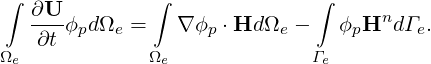 | (15.2) |
The fluxes are calculated at some quadrature points and a quadrature rule with NQ quadrature points is adopted to calculate the integration in the element and NQΓ quadrature points on element boundaries. This leads to
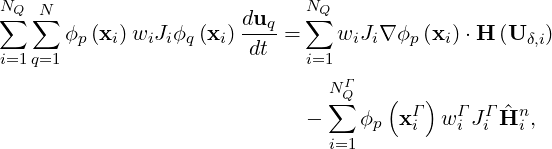 | (15.3) |
where uq is the coefficient vector of the basis function. The whole discretization can be written in the following matrix form
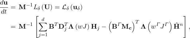 | (15.4) |
where d is the spatial dimension, M = BT Λ B is the mass matrix, Λ represents a
diagonal matrix, Dj is the derivative matrix in the jth direction, BΓ is the backward
transformation matrix of ϕΓ and Mc is the mapping matrix between ϕΓ and ϕ, J is the
interpolation matrix from quadrature points of a element to quadrature points of its element
boundaries.
B is the mass matrix, Λ represents a
diagonal matrix, Dj is the derivative matrix in the jth direction, BΓ is the backward
transformation matrix of ϕΓ and Mc is the mapping matrix between ϕΓ and ϕ, J is the
interpolation matrix from quadrature points of a element to quadrature points of its element
boundaries.
The weak DG scheme for the advection term is complete as long as a Riemann numerical flux
is used to calculate the normal flux,  n
n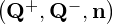 , in which Q+ and Q- are variable values
on the exterior and interior sides of the element boundaries, respectively. Similarly, LDG or IP
methods are needed to provide the numerical fluxes on element boundaries for the diffusion
terms.
, in which Q+ and Q- are variable values
on the exterior and interior sides of the element boundaries, respectively. Similarly, LDG or IP
methods are needed to provide the numerical fluxes on element boundaries for the diffusion
terms.
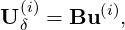
Various multi-step and multi-stage methods have been implemented in an object-oriented general linear methods framework. Here, the Runge-Kutta methods are took as examples. The ith stage of the Runge-Kutta method is
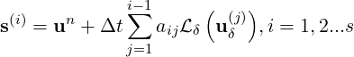 | (15.5) |
 | (15.6) |
 | (15.7) |
where aij is the coefficient of the Runge-Kutta method, s is a source term, B is the backward transform matrix. Finally, the solution of the new time step (n + 1) is calculated by
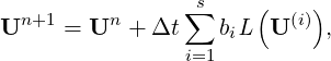 | (15.8) |
For explicit RK methods, aii = 0, the discretization is complete and straightforward.
Eq. (15.6) of the implicit stages (aii≠0) can be written as the nonlinear system
 | (15.9) |
This system is iteratively solved by Newton’s method [46] with the Newton step, Δv = vk+1 -vk, updated through the solution of the linear system
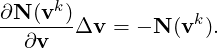 | (15.10) |
where v0 = s(i) is adopted as an initial guess. When the Newton residual is smaller than the convergence tolerance of the Newton iterations τ, which is
 | (15.11) |
uit(i) = vk is regarded as the approximate solution of the nonlinear system, where R is the remaining Newton residual vector N(uit(i)) after convergence.
The restarted generalized minimal residual method (GMRES) [56] is used for solving the linear problem (15.10). The Jacobian matrix and vector inner product operator is approximated by the following finite difference
 | (15.12) |
where ϵ is the step size of the finite difference approximation.
The use of good preconditioners in GMRES is very important for efficiently solving stiff linear systems. Instead of solving the system of Eq. (15.10) directly, one can get the same solution by solving the preconditioned linear system
 | (15.13) |
where P is the preconditioning matrix. A low memory block relaxed Jacobi iterative preconditioner is implemented.