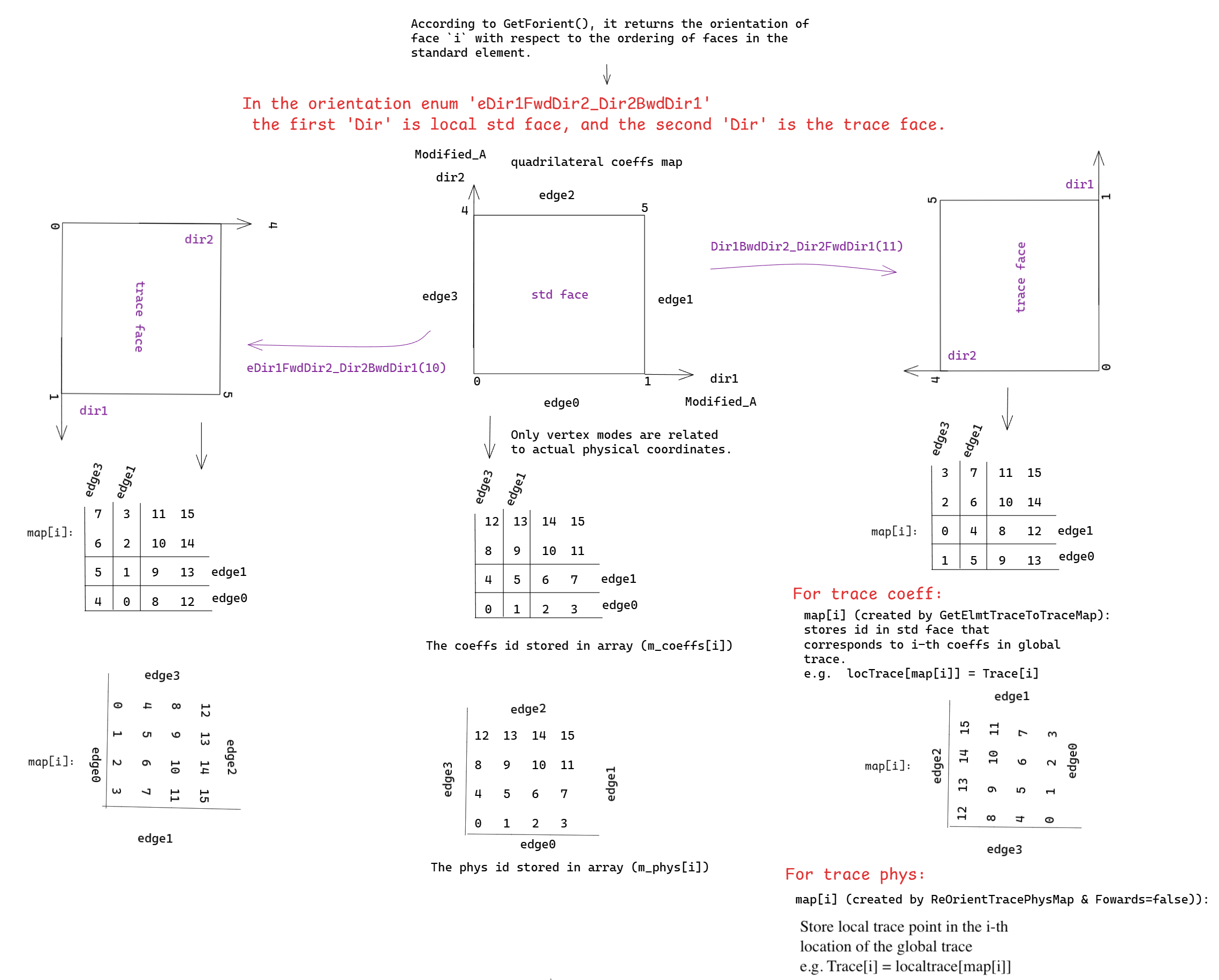
Figure 7.3 Example of trace mappings for complex transposed cases
eDir1FwdDir2_Dir2BwdDir1 and eDir1BwdDir2_Dir2FwdDir1.
As stated in the introduction, this section of this guide is structured in question-answer form. This is not meant to capture every possible question asked of us on the Nektar++ users list; however, this set of (ever-growing) questions are meant to capture the “big ideas” that developers want to know about how LocalRegions work and how they can be used.
In this section, we will through question and answer format try to cover the following basic algorithmic concepts that are found within the LocalRegions part of the library:
When handling discontinuous Galkerin (DG) expansions and techniques such as Gradient Jump Penalisation we need to be able to take data from the trace of the element (i.e. edges in 2D elements and faces in 3D element) to a unique trace which is shaped between two elements. This is necessary for example to perform a Riemann problem to link two elements in DG field. Such an action might require interpolation from one distribution of quadrature points to another however the shared trace space may not be aligned trivially with the element trace.
In two-dimensions we only have edges which are either aligned so that the local coordinate
system runs in the same direction, noted by the enum StdRegions::eForwards in the
code, or in reverse direction, noted by the enum StdRegions::eBackwards in the
code.
In three-dimensions the mappings get more complicated particularly for quadrilateral faces.
For triangular faces, our use of the collapsed coordinate system means that triangular faces
can only align in a forwards or backwards sense because the singular vertices must align and
so this is managed in the mesh generation stage. For a triangular faces we use the enum
StdRegions::eDir1FwdDir1_Dir2FwdDir2 to denote a forwards aligned face and the enum
StdRegions::eDir1BwdDir1_Dir2FwdDir2 to denote a face where the bottom x-coordinate
runs in the reverse of backwards direction on the element trace compared to the shared
trace.
At this point the meaning of the face enums needs a bit more explanation. For any
two-dimensional trace we have two coordinates which are denoted by “Dir1”
(Direction 1, i.e. x-direction) and “Dir 2” (Direction 2, i.e. y-direction). So the num
StdRegions::eDir1FwdDir1_Dir2FwdDir2 denotes that direction 1 of the original triangle (or
quadrilateral) is aligned to direction 1 of the shared/mapped triangle (or quadrilateral) and
the two direction are aligned (i.e. Forwards). It also denotes that direction 2 of the original
triangle (or quadrilateral) is aligned to direction 2 of the shared/mapped triangle (or
quadrilateral). The enum StdRegions::eDir1BwdDir1_Dir2FwdDir2 is similarly interpreted
but Direction 1 of the original face is now aligned to be in the reverse direction to Direction 1
of the shared/mapped face.
For quadrilateral faces there are eight possible permutatiions that one quadrilateral can be oriented to another quadrilateral and these include
StdRegions::eDir1FwdDir1_Dir2FwdDir2
StdRegions::eDir1FwdDir1_Dir2BwdDir2
StdRegions::eDir1BwdDir1_Dir2FwdDir2
StdRegions::eDir1BwdDir1_Dir2BwdDir2
StdRegions::eDir1FwdDir2_Dir2FwdDir1
StdRegions::eDir1FwdDir2_Dir2BwdDir1
StdRegions::eDir1BwdDir2_Dir2FwdDir1
StdRegions::eDir1BwdDir2_Dir2BwdDir1
When coding we typically want to match the coefficients or physical quadrature points from
one face to another and so there are methods to produce the mapping arrays to achieve this.
For quadrature points we have Expansion3D::ReOrientTracePhysMaps(). In most cases
there is a symmetry as to whether you map from the element trace to the shared
trace or vice versa but for the two cases StdRegions::eDir1FwdDir2_Dir2BwdDir1
StdRegions::eDir1BwdDir2_Dir2FwdDir1 where the faces are transposed and one direction is
reversed care must be taken since the mappings are not symmetric. The method
Expansion3D::ReOrientTracePhysMaps() is defined by default to provide a mapping which
takes the local trace to the global trace such that sharedtrace[i] = localtrace[map[i]].
However it is possible to provide a false boolean to the argument Forwards and it will
return the mapping from the shared trace to the local trace so that localtrace[i] =
sharedtrace[map[i]].
Figure 7.3 provides an example of this more complex mapping case for the reordering of the face coefficients and also highlights the changes in the face orientation.
With the big ideas in place, let us now start into our questions.