Most of the solvers in Nektar++, including the incompressible Navier-Stokes equations, rely on the solution of a Helmholtz equation,
| (9.1) |
an elliptic boundary value problem, at every time-step, where u is defined on a domain Ω of Nel non-overlapping elements. In this section, we outline the preconditioners which are implemented in Nektar++. Whilst some of the preconditioners are generic, many are especially designed for the modified basis only.
The standard spectral/hp approach to discretise (9.1) starts with an expansion in terms of the elemental modes:
| (9.2) |
where Nel is the number of elements, Nme is the number of local expansion modes within the element Ωe, ϕne(x) is the nth local expansion mode within the element Ωe, ûne is the nth local expansion coefficient within the element Ωe. Approximating our solution by (9.2), we adopt a Galerkin discretisation of equation (9.1) where for an appropriate test space V δ we find an approximate solution uδ ∈ V δ such that

This can be formulated in matrix terms as

where H represents the Helmholtz matrix,  are the unknown global coefficients and f the
inner product the expansion basis with the forcing function.
are the unknown global coefficients and f the
inner product the expansion basis with the forcing function.
We first consider the C0 (i.e. continuous Galerkin) formulation. The spectral/hp expansion basis is obtained by considering interior modes, which have support in the interior of the element, separately from boundary modes which are non-zero on the boundary of the element. We align the boundary modes across the interface of the elements to obtain a continuous global solution. The boundary modes can be further decomposed into vertex, edge and face modes, defined as follows:
vertex modes have support on a single vertex and the three adjacent edges and faces as well as the interior of the element;
edge modes have support on a single edge and two adjacent faces as well as the interior of the element;
face modes have support on a single face and the interior of the element.
When the discretisation is continuous, this strong coupling between vertices, edges and faces leads to a matrix of high condition number κ. Our aim is to reduce this condition number by applying specialised preconditioners. Utilising the above mentioned decomposition, we can write the matrix equation as:
![⌊ ⌋ ⌊ ⌋
[ H H ] ^ub ^fb
bb bi |⌈ ^ui |⌉ = |⌈ ^fi |⌉
Hib Hii](developer-guide144x.svg)
where the subscripts b and i denote the boundary and interior degrees of freedom respectively. This system then can be statically condensed allowing us to solve for the boundary and interior degrees of freedom in a decoupled manor. The statically condensed matrix is given by
![[ ]⌊ ⌋ ⌊ -1 ⌋
Hbb - HbiH -1Hib 0 | ^ub | | ^fb - HbiH ii ^fi |
H ii H ⌈ ^ui ⌉ = ⌈ ^fi ⌉
ib ii](developer-guide145x.svg)
This is highly advantageous since by definition of our interior expansion this vanishes on the boundary, and so Hii is block diagonal and thus can be easily inverted. The above sub-structuring has reduced our problem to solving the boundary problem:

where S1 = Hbb -HbiHii-1Hib and  1 =
1 =  b -HbiHii-1
 i. Although this new system typically
has better convergence properties (i.e lower κ), the system is still ill-conditioned, leading to a
convergence rate of the conjugate gradient (CG) routine that is prohibitively slow. For this
reason we need to precondition S1. To do this we solve an equivalent system of the
form:
i. Although this new system typically
has better convergence properties (i.e lower κ), the system is still ill-conditioned, leading to a
convergence rate of the conjugate gradient (CG) routine that is prohibitively slow. For this
reason we need to precondition S1. To do this we solve an equivalent system of the
form:

where the preconditioning matrix M is such that κ is less than κ
 and
speeds up the convergence rate. Within the conjugate gradient routine the same
preconditioner M is applied to the residual vector
and
speeds up the convergence rate. Within the conjugate gradient routine the same
preconditioner M is applied to the residual vector  k+1 of the CG routine every
iteration:
k+1 of the CG routine every
iteration:

When utilising a hybridizable discontinuous Galerkin formulation, we perform a static condensation approach but in a discontinuous framework, which for brevity we omit here. However, we still obtain a matrix equation of the form

where Λ represents an operator which projects the solution of each face back onto the
three-dimensional element or edge onto the two-dimensional element. In this setting then,  consists of degrees of freedom for each egde (in 2D) or face (in 3D). The overall system does
not, therefore, results in a weaker coupling between degrees of freedom, but at the expense of
a larger matrix system.
consists of degrees of freedom for each egde (in 2D) or face (in 3D). The overall system does
not, therefore, results in a weaker coupling between degrees of freedom, but at the expense of
a larger matrix system.
Within the Nektar++ framework a number of preconditioners are available to speed up the convergence rate of the conjugate gradient routine. The table below summarises each method, the dimensions of elements which are supported, and also the discretisation type support which can either be continuous (CG) or discontinuous (hybridizable DG).
| Name | Dimensions | Discretisations |
Null | All | All |
Diagonal | All | All |
FullLinearSpace | 2/3D | CG |
LowEnergyBlock | 3D | CG |
Block | 2/3D | All |
LOR | 2/3D | CG |
FullLinearSpaceWithDiagonal | All | CG |
FullLinearSpaceWithLowEnergyBlock | 2/3D | CG |
FullLinearSpaceWithBlock | 2/3D | CG |
The default is the Diagonal preconditioner. The above preconditioners are specified through
the Preconditioner option of the SOLVERINFO section in the session file. For example, to
enable FullLinearSpace one can use:
1 <I PROPERTY="Preconditioner" VALUE="FullLinearSpace" />
Alternatively one can have more control over different preconditioners for each solution field
by using the GlobalSysSoln section. For more details, consult the user guide. The following
sections specify the details for each method.
Diagonal (or Jacobi) preconditioning is amongst the simplest preconditioning strategies. In this scheme one takes the global matrix H = (hij) and computes the diagonal terms hii. The preconditioner is then formed as a diagonal matrix M-1 = (hii-1).
The linear space (or coarse space) of the matrix system is that containing degrees of freedom corresponding only to the vertex modes in the high-order system. Preconditioning of this space is achieved by forming the matrix corresponding to the coarse space and inverting it, so that

Since the mesh associated with higher order methods is relatively coarse compared with traditional finite element discretisations, the linear space can usually be directly inverted without memory issues. However such a methodology can be prohibitive on large parallel systems, due to a bottleneck in communication.
In Nektar++ the inversion of the linear space present is handled using the XXT library. XXT
is a parallel direct solver for problems of the form A =
=  based around a sparse factorisation
of the inverse of A. To precondition utilising this methodology the linear sub-space is gathered
from the expansion and the preconditioned residual within the CG routine is determined by
solving
based around a sparse factorisation
of the inverse of A. To precondition utilising this methodology the linear sub-space is gathered
from the expansion and the preconditioned residual within the CG routine is determined by
solving
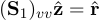
The preconditioned residual  is then scattered back to the respective location in the global
degrees of freedom.
is then scattered back to the respective location in the global
degrees of freedom.
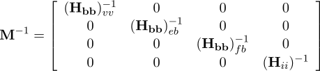
Block preconditioning of the C0 continuous system is defined by the following:
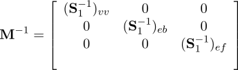
where diag[(S1)vv] is the diagonal of the vertex modes, (S1)eb and (S1)fb are block diagonal matrices corresponding to coupling of an edge (or face) with itself i.e ignoring the coupling to other edges and faces. This preconditioner is best suited for two dimensional problems.
In the HDG system, we take the block corresponding to each face and invert it. Each of these inverse blocks then forms one of the diagonal components of the block matrix M-1.
Applied to the full matrix system H, the preconditioner additionally includes the inverse of the interior modes Hii and is defined by:
Low energy basis preconditioning follows the methodology proposed by Sherwin & Casarin. In this method a new basis is numerically constructed from the original basis which allows the Schur complement matrix to be preconditioned using a block preconditioner. The method is outlined briefly in the following.
Elementally the local approximation uδ can be expressed as different expansions lying in the same discrete space V δ

Since both expansions lie in the same space it’s possible to express one basis in terms of the other via a transformation, i.e.

Applying this to the Helmholtz operator it is possible to show that,

For sub-structured matrices (S) the transformation matrix (C) becomes:
![[ ]
R 0
C = 0 I](developer-guide167x.svg)
Hence the transformation in terms of the Schur complement matrices is:

Typically the choice of expansion basis ϕ1 can lead to a Helmholtz matrix that has undesirable properties i.e poor condition number. By choosing a suitable transformation matrix C it is possible to construct a new basis, numerically, that is amenable to block diagonal preconditioning.
![⌊ ⌋ [ ]
| SvvT Sve Svf | Svv Sv,ef
S1 = ⌈ S veT SeeT Sef ⌉ = ST Sef,ef
S vf S ef Sff v,ef](developer-guide169x.svg)
Applying the transformation S2 = RS1RT leads to the following matrix
![[ T T T T ]
S = Svv + RvS v,ef + Sv,efR v + RvSef,efR v [Sv,ef + RvSef,ef]A
2 A[STv,ef + Sef,efRTv ] ASef,efAT](developer-guide170x.svg)
where ASef,efAT is given by
![[ T T T ]
AS AT = See + Ref Sef + SefR ef + RefSffR ef Sef + RefSff
ef,ef STef + Sff RTef Sff](developer-guide171x.svg)
To orthogonalise the vertex-edge and vertex-face modes, it can be seen from the above that
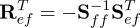
and for the edge-face modes:

Here it is important to consider the form of the expansion basis since the presence of Sff-1 will lead to a new basis which has support on all other faces; this is problematic when creating a C0 continuous global basis. To circumvent this problem when forming the new basis, the decoupling is only performed between a specific edge and the two adjacent faces in a symmetric standard region. Since the decoupling is performed in a rotationally symmetric standard region the basis does not take into account the Jacobian mapping between the local element and global coordinates, hence the final expansion will not be completely orthogonal.
The low energy basis creates a Schur complement matrix that although it is not completely orthogonal can be spectrally approximated by its block diagonal contribution. The final form of the preconditioner is:
![⌊ ⌋-1
| diag[(S2)vv] 0 0 |
M - 1 = || 0 (S2)eb 0 ||
⌈ 0 0 (S2)fb ⌉](developer-guide174x.svg)
where diag[(S2)vv] is the diagonal of the vertex modes, (S2)eb and (S2)fb are block diagonal matrices corresponding to coupling of an edge (or face) with itself i.e ignoring the coupling to other edges and faces.
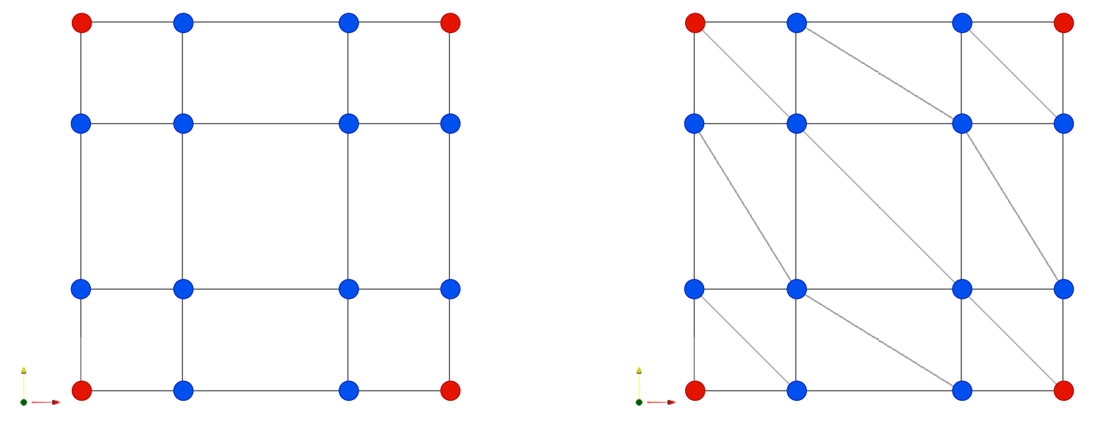
For the construction of the LOR preconditioner, the global matrix H is interpolated from the higher-order spectral/hp discretisation to its corresponding low-order (P=1) “refined" finite element discretisation HL. The conceptual representation of this conversion is seen in Fig. 9.4, where the LOR mesh on the right is a sub-structured grid of collocated Gauss-Lobatto-Legendre (GLL) nodal points. The application of the preconditioning matrix M is then formulated as M-1 = HL-1.
For the high-order discretisation H, every internal DOF is coupled with every other DOF in an element. The conversion to the LOR space HL increases the sparsity as now the DOF are only connected to their immediate neighbours. The difference in connectivity between the two discretisations is further accentuated in mathematical operators, even if the number of DOF is the same (as seen in Fig. 9.4). Thus, the operators on the lower-order discretisation are cheaper to evaluate than their higher-order counterparts.
The generalised Vandemonde matrix V from Eqn. (9.3) is used for the interpolation of the higher-order polynomial space to the collocated Lagrange basis in the LOR space. In matrix terms, this interpolation is expressed as,
| (9.3) |
where, f[i] = f(ξi) is the known polynomial expansion, V[i][j] = ϕj(ξi) where ϕj is the chosen
basis function and  [j] =
[j] =  (ξj) are the unknown expansion coefficients. The unknown Lagrange
polynomials are then found using
(ξj) are the unknown expansion coefficients. The unknown Lagrange
polynomials are then found using  = V-1f. The interpolation basis works for any basis
selection in the HO space, where the matrix V is appropriately constructed according
to the choice of higher-order expansion basis [?]. The interpolation for the case of
the nodal expansion corresponds to a collocation projection. In contrast, a modal
expansion basis is more involved as the construction of V has to handle the change of
basis. The interpolation step is applied to both the trial and test functions in the
higher-order polynomial space, and the interpolated functions are then used to construct
HL.
= V-1f. The interpolation basis works for any basis
selection in the HO space, where the matrix V is appropriately constructed according
to the choice of higher-order expansion basis [?]. The interpolation for the case of
the nodal expansion corresponds to a collocation projection. In contrast, a modal
expansion basis is more involved as the construction of V has to handle the change of
basis. The interpolation step is applied to both the trial and test functions in the
higher-order polynomial space, and the interpolated functions are then used to construct
HL.
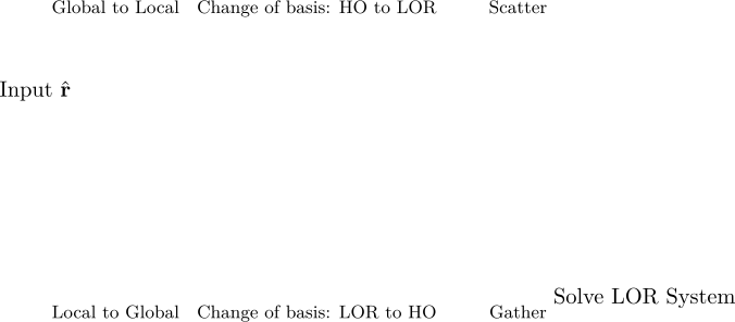
Fig. 9.5 gives an overview of the Nektar++ LOR preconditioner algorithm.
The following steps are done for the preconditioning:
The input to the LOR preconditioner code is the residual of the iterative solution
 at a given iteration (like all other preconditioners in Nektar++).
The LOR space (HL) is
generated at the PreconditionerLOR::v_BuildPreconditioner step, using the
MeshGraph::LinearMeshGraph method. This method has further setups to handle
the
LOR space for each element type (LinMeshSetUp1DGeom, LinMeshSetUp2DGeom,
LinMeshSetUpTetGeom, LinMeshSetUpPrismGeom). A coefficient map (m_ho2lor)
is also generated during this step to handle the transformations between HO and
LOR spaces and vice versa.
Interpolation of the solution from the HO discretization to the LOR space is
performed using an appropriately constructed generalized Vandermonde matrix V,
which depends on the choice of the higher-order expansion basis (MODIFIED or
GLL_LAGRANGE). This interpolation is managed by MultiplyByBlockMatrix
operations in the PreconditionerLOR::v_DoPreconditioner routine. Special
keys (eGLLToCoeffs and eEquiSpacedToCoeffs) and their implementations are
defined in the ExpList and StdExpansion classes to handle this process.
After
interpolating to the LOR space, the linear system is solved using an appropriate
inner-iteration strategy. This is done using m_LORLinSys->SolveLinearSystem
within PreconditionerLOR::v_DoPreconditioner.
The solution from the LOR mesh is then mapped back to the HO space and subsequently transformed onto the original expansion basis by applying the inverse of the V matrix operation. Essentially, this reverses the steps taken before solving the LOR system.
Appropriate scatter-gather transformations are handled using the assembly maps
(m_ho2lor) in both spaces.
The choice of discretisation in the LOR space has a bearing on the conditioning properties of
the LOR preconditioner. There are two options for the point distribution in the LOR
space - equispaced and GLL distribution. The GLL distribution is consistent with
the spectral equivalence of the HO-LOR spaces. Still, the former option is solely
available to test the preconditioner performance for an equidistant point spacing. The
default point distribution for the LOR preconditioner is GLL distribution. It can be
activated using the property LORPointDistribution, with the options GLL and
Equispaced.
There are two options to discretise the quadrilaterals in the LOR space in the Nektar++ implementation following the work of Canuto [16], namely Q1 and P1 elements. The differences can be seen in Figure 9.6, where for a given quadrilateral element at a fixed polynomial order the GLL points in the LOR space can either be formulated with Q1 (quadrilateral) elements or P1 (triangular) elements.
Notice that there can be many possible orientations for P1 elements, and the choice in Figure
9.6 is one such possibility. There are no such options for triangular elements in the LOR
space as they can only be discretised in further smaller P1 elements. It can be activated using
the property LORSimplex, with the options False for Q1 (default) and True for
P1.
The LOR discretisation for triangles requires a different strategy. For a nodal expansion in triangles, that a closed-form expression for Lagrange polynomial does not exist like in the case of tensorial product of modal expansions for Gauss-Lobatto-Legendre (GLL) nodal points. Thus, the formation of LOR space, which is always a grid of collocated nodal points, can’t be created in a straightforward manner for triangles with either choice of higher-order expansion basis and requires shifting the problem to electrostatic points (ξele). The problem is interpolated to the LOR space after this shift. The visualisation of the process is seen in Figure 9.7, but in reality the construction of the generalised Vandemonde matrix V takes care of this shift of basis operation.
Tetrahedrons and Prisms follow a similar approach for the construction of the LOR space. The visualisation of this construction is seen in Fig. 9.8. Fig. 9.7a and 9.7b show the LOR space for tetrahedrons at P = 3 and 6. Fig. 9.7c and 9.7d show the LOR space for prisms at P = 3 and 6, where a prismatic domain expansion is achieved by extending the triangular nodal expansion by making a tensor product with the Lagrange polynomial in the third direction.
LOR preconditioner provides various options to setup and solve the preconditioned system.
These settings work when the GLOBALSYSSOLNINFO has:
1  <I PROPERTY="GlobalSysSoln"             VALUE="IterativeFull" />
2  <I PROPERTY="Preconditioner"            VALUE="LOR" />
3  <I PROPERTY="LinSysIterSolver"          VALUE="GMRES" />
The full list is found below:
1    <I PROPERTY="GlobalSysSoln"             VALUE="IterativeFull" />
2    <I PROPERTY="Preconditioner"            VALUE="LOR"/>
3    <I PROPERTY="LinSysIterSolver"          VALUE="GMRES" />
4    <I PROPERTY="LORSolverType"             VALUE="DirectFull" />
5    <I PROPERTY="LORPointDistribution"      VALUE="GLL" />
6    <I PROPERTY="LORSimplex"                VALUE="False" />
LORSolverType - The type of solver to use for the inner iteration in the LOR
preconditioner, i.e. working on the LOR mesh. most commonly used are DirectFull,
PETScFull. Rest are quite experimental, and do not give great performance. They have
not been tested extensively in 3D. Options:
DirectFull: Direct solve on Ax = b. Use this with caution when your problem
size is greater than 2000 DOF.
XxtFull: Parallel direct solve on Ax = b. Not well tested.
IterativeFull: Apply available native linear solvers to solve the LOR system.
Preconditioner: Option to further apply a preconditioner on the LOR mesh.
LORPointDistribution - Options: GLL (default), Equispaced
LORSimplex - Options: True means P1 type element for quads in the LOR space, False
means Q1 type element
The following options are available when LORSolverType = IterativeFull
LORLinSysIterSolver: Options: All available native linear solvers in Nektar++.
Default: ConjugateGradient.
LORPreconditioner: Applying a further preconditioner on the LOR space.
Default: Diagonal.
LORFixedIterations: Applying a fixed number of iterations on the
LORLinSysIterSolver.
LORIterativeTolerance: The tolerance for the inner loop solver in the LOR
preconditioner.
Example:
1  <I PROPERTY="LORLinSysIterSolver"    VALUE="GMRES" />
2  <I PROPERTY="LORPreconditioner"    VALUE="FullLinearSpace" />
3  <I PROPERTY="LORFixedIterations"        VALUE="06" />
4  <I PROPERTY="LORIterativeTolerance"      VALUE="1e-4" />
To use the AMG solver from BoomerAMG to solve the LOR system when LORSolverType =
PETScFull, we advise the following settings:
For one V-cycle of BoomerAMG at every iteration (efficient for large 3D cases)
1-ksp_type preonly
2-pc_type hypre
3-pc_hypre_type boomeramg
4-pc_hypre_boomeramg_max_iter 1
For applying multiple V-cycles to solve under a certain tolerance (reduces outer iterations, but can be time consuming for large cases)
1-ksp_rtol 1e-4 #choose your tolerance, keep it high
2-ksp_type richardson
3-pc_type hypre
4-pc_hypre_type boomeramg
Reliable set of AMG settings for BoomerAMG for non-symmetric Poisson system resulting from LOR discretisation.
1-pc_hypre_boomeramg_coarsen_type hmis
2-pc_hypre_boomeramg_relax_type_all sor/jacobi
3-pc_hypre_boomeramg_grid_sweeps_all 2
4-pc_hypre_boomeramg_strong_threshold 0.7 #0.25 for 2D cases
5-pc_hypre_boomeramg_interp_type ext+i
6-pc_hypre_boomeramg_P_max 2
7-pc_hypre_boomeramg_truncfactor 0.3