 = f(t,y), y(t0) = y0
This directory consists of the following primary files:
| TimeIntegrationScheme.h | TimeIntegrationScheme.cpp |
| TimeIntegrationGLM.h | TimeIntegrationGLM.cpp |
| *TimeIntegrationSchemes.h | Specific GLM schemes, e.g. AB, RK, IMEX, etc. |
| TimeIntegrationFIT.h | TimeIntegrationFIT.cpp |
| TimeIntegrationGEM.h | TimeIntegrationGEM.cpp |
| TimeIntegrationSDC.h | TimeIntegrationSDC.cpp |
The original time-stepping interface (found in the parent class TimeIntegrationScheme) where implemented by Vos et al. [69] and a detailed explanation of the mathematics and computer science concepts are provided there. After the original implementation, the time-stepping routines were refactored into a factory pattern (found in the child class TimeIntegrationGLM with specific GLM schemes covering both traditional and exponential schemes (compartmentalize in the *TimeIntegrationSchemes classes). Each GLM scheme sets up one or more (linear multistep methods) phases using the TimeIntegrationAlgorithmGLM class, which is where the GLM algorithm is performed using the helper class TimeIntegrationSolutionGLM.
More recently Extrapolation, Spectral-Deferred-Correction, and Fractional-in-time schemes have been added as sibbling classes to the GLM class (found in the child classes TimeIntegrationGEM, TimeIntegrationSDC, and TimeIntegrationFIT, respectively). The Extrapolation, Spectral-Deferred-Correction, and the Fractional-in-time schemes make use of their own separate algorithm.
General linear methods (GLMs) can be considered as the generalization of a broad range of different numerical methods for ordinary differential equations. They were introduced by Butcher and they provide a unified formulation for traditional methods such as the Runge-Kutta methods and the linear multi-step methods such as Adams-Bashforth. From an implementation point of view, all these numerical methods can be abstracted similarly and allows a high level of generality which is the case in Nektar++. For background information about general linear methods, see [14].
The standard initial value problem can written in the form
| = f(t,y), y(t0) = y0 |
where y is a vector containing the variable (or an array of array containing the variables).
In the formulation of general linear methods, it is more convenient to consider the ODE in autonomous form, i.e.
 = ^ f (^y ), ^ y (t0) = ^ y 0. = ^ f (^y ), ^ y (t0) = ^ y 0. |
Suppose the governing differential equation is given in autonomous form, the nth step of the GLM comprising
is formulated as:
| Y i | = Δt∑ j=0s-1a ijFj + ∑ j=0r-1u ij^ y j[n-1], i = 0,1,…,s - 1 | ||
| ^y i[n] | = Δt∑ j=0s-1b ijFj + ∑ j=0r-1v ij^ y j[n-1], i = 0,1,…,r - 1 |
where Y i are referred to as the stage values and Fj as the stage derivatives. Both quantities are related by the differential equation:
| Fi = ^ f (Y i). |
The matrices A = [aij], U = [uij], B = [bij], V = [vij] are characteristic of a specific method. Each scheme can then be uniquely defined by a partitioned (s + r) × (s + r) matrix
![[ ]
A U
B V](developer-guide14x.png) |
Adopting the notation:
^y [n-1] = ![⌊ [n-1] ⌋
| y^0 |
|| y^[n1-1] ||
|| .. ||
⌈ . ⌉
y^[nr--11]](developer-guide15x.png) , ^ y [n] = , ^ y [n] = ![⌊ [n] ⌋
| ^y0 |
|| ^y[n1] ||
|| .. ||
⌈ . ⌉
^y[rn-]1](developer-guide16x.png) , Y = , Y = 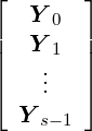 , F = , F = 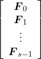 |
the general linear method can be written more compactly in the following form:
![[ Y ]
[n]
^y](developer-guide19x.png) = = ![[ A ⊗ I U ⊗ I ]
N N
B ⊗ IN V ⊗ IN](developer-guide20x.png) ![[ ΔtF ]
[n-1]
y^](developer-guide21x.png) |
where IN is the identity matrix of dimension N × N.
Although the GLM is essentially presented for ODE’s in its autonomous form, in Nektar++ it will be used to solve ODE’s formulated in non-autonomous form. Given the ODE,
 = f(t,y), y(t0) = y0 = f(t,y), y(t0) = y0 |
a single step of GLM can then be evaluated in the following way:
y[n-1], i.e. the r subvectors comprising yi[n-1] - t[n-1], i.e. the equivalent of y[n-1] for the time variable t.
For a detailed description of the formulation and a deeper insight of the numerical method see [69].
Nektar++ contains various classes and methods which implement the concept of GLMs. This toolbox is capable of numerically solving the generalised ODE using a broad range of different time-stepping methods. We distinguish the following types of general linear methods:
where φ0(z) = ez for k = 0, φk(z) = 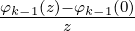 for k ≥ 1.
While implemented, exponential schemes are not currently seeded.
The aim in Nektar++ is to fully support the first three types of GLMs. Fully implicit methods are currently not implemented.
In addition to the GLMs Nektar++ also supports extrapolation methods:
The Extrapolation methods follow the same paradigm as the GLMs, that is both have the same parent class and as such have the same interface.
For more details about Extrapolation methods, interested readers can refer to [25].
In addition to the GLMs Nektar++ also supports extrapolation methods:
The Extrapolation methods follow the same paradigm as the GLMs, that is both have the same parent class and as such have the same interface.
For more details about Extrapolation methods, interested readers can refer to [25].
In addition to the GLMs Nektar++ also supports spectral deferred correction methods:
The Spectral Deferred Correction methods follow the same paradigm as the GLMs, that is both have the same parent class and as such have the same interface.
For more details about Spectral Deferred Correction methods, interested readers can refer to [30, 56, 47].
In addition to the GLMs Nektar++ also supports fractional methods:
The Fractional methods follow the same paradigm as the GLMs, that is both have the same parent class and as such have the same interface.
The goal of abstracting the concept of general linear methods and fractional methods is to provide users with a single interface for time-stepping, independent of the chosen method. The classes tree allows the user to numerically integrate ODE’s using high-order complex schemes, as if it was done using the Forward-Euler method. Switching between time-stepping schemes is as easy as changing a parameter in an input file.
In the already implemented solvers the time-integration schemes have been set up according to the nature of the equations. For example the incompressible Navier-Stokes equations solver allows the use of three different Implicit-Explicit time-schemes if solving the equations with a splitting-scheme. This is because this kind of scheme has an explicit and an implicit operator that combined solve the ODE’s system.
Once aware of the problem’s nature and implementation, the user can easily switch between some (depending on the problem) of the following time-integration schemes:
| Method | Variant | Order / Free Parameters |
| ForwardEuler |
| Forward-Euler scheme |
| BackwardEuler |
| Backward-Euler scheme |
| AdamsBashforth |
| Adams-Bashforth Forward multi-step scheme of order 1-4 |
| AdamsMoulton |
| Adams-Moulton Forward multi-step scheme of order 1-4 |
| BDFImplicit |
| BDF multi-step implicit scheme of order 1-4 |
| RungeKutta |
| Runge-Kutta multi-stage explicit scheme of order 1-5, (2 - midpoint, 3 - Ralston’s, 4 - Classic) |
| RungeKutta | SSP | Strong Stability Preserving (SSP) variant of the RungeKutta multi-stage explicit scheme of order 1-3 |
| DIRK |
| Diagonally Implicit Runge-Kutta (DIRK) scheme of order 2-3 |
| CNAB |
| Crank-Nicolson-Adams-Bashforth (CNAB) of order 2 |
| MCNAB |
| Modified Crank-Nicolson-Adams-Bashforth (MCNAB) of order 2 |
| IMEX |
| Implicit-Explicit (IMEX) scheme using Backward Different Formula Extrapolation of order 1-4 |
| IMEX | Gear | IMEX Gear variant of order 2 |
| IMEX | dirk | IMEX DIRK variant with free parameters (s, sigma), where s is the number of implicit stage schemes, sigma is the number of explicit stage scheme and p is the combined order of the scheme (Note: IMEX DIRK schemes should not be used with IncNavierStokesSolver). |
|
| dirk | Forward-Backward Euler, first order, free parameters (1,1) |
|
| dirk | Forward-Backward Euler, first order, free parameters (1,2) |
|
| dirk | Implicit-Explicit Midpoint, second order, free parameters (1,2) |
|
| dirk | L-stable, two stage, second order, free parameters (2,2) |
|
| dirk | L-stable, two stage, second order, free parameters (2,3) |
|
| dirk | L-stable, two stage, third order, free parameters (2,3) |
|
| dirk | L-stable, three stage, third order, free parameters (3,4) |
|
| dirk | L-stable, four stage, third order, free parameters (4,4) |
| EulerExponential | Lawson | Exponential Euler scheme using the Lawson variant of order 1 |
|
| Nørsett | Exponential Euler scheme using the Nørsett variant of order 1-4 (Higher order not yet properly seeded) |
| ExtrapolationMethod | ExplicitEuler | Extrapolation method of arbitrary order using a series of first-order explict Euler scheme |
|
| ExplicitMidpoint | Extrapolation method of arbitrary order using a series of second-order explict midpoint scheme |
|
| ImplicitEuler | Extrapolation method of arbitrary order using a series of first-order implicit Euler scheme |
|
| ImplicitMidpoint | Extrapolation method of arbitrary order using a series of second-order implicit Euler scheme |
| ExplicitSDC | Equidistant | Explicit Spectral Deferred Correction method of arbitrary order using equidistant quadrature points and first-order explicit Euler schemes |
|
| GaussLobattoChebyshev | Explicit Spectral Deferred Correction method of arbitrary order using Gauss-Lobatto-Chebyshev quadrature points and first-order explicit Euler schemes |
|
| GaussLobattoLegendre | Explicit Spectral Deferred Correction method of arbitrary order using Gauss-Lobatto-Legendre quadrature points and first-order explicit Euler schemes |
|
| GaussRadauChebyshev | Explicit Spectral Deferred Correction method of arbitrary order using Gauss-Radau-Chebyshev quadrature points and first-order explicit Euler schemes |
|
| GaussRadauLegendre | Explicit Spectral Deferred Correction method of arbitrary order using Gauss-Radau-Legendre quadrature points and first-order explicit Euler schemes |
| ImplicitSDC | GaussRadauLegendre | Implicit Spectral Deferred Correction method of arbitrary order using Gauss-Radau-Legendre quadrature points and first-order implicit Euler schemes |
| FractionalInTime |
| Fractional-in-time scheme of order 1-4 (Higher order not yet properly seeded), free parameters, none, one (alpha), two (alpha, base), or six (alpha, base, nQuadPts, sigma, mu0, nu) |
Note: in many cases the first order schemes reduce to either a forward or backward Euler scheme.
Nektar++ input file for your problem will require a string corresponding to the time-stepping
method and the order, and optionally the variant and free parameters. In addition, parameters
that define your integration in time, the time-step and number of steps or final time. For
example:
The old schema which specified the method, variant, order, and free parameters as a single string has been deprecated but remains backwards compatible.
In order to implement a new solver which takes advantage of the time-integration class in Nektar++, two main ingredients are required:
Your pseudo-main file, where you actually loop over the time steps, will look like
We can distinguish three different sections in the code above
In this section you define the basic parameters (like time-step, initial time, etc.) and the
time-integration objects. The operators are not all required, it depends on the nature of your
problem and on the type of time integration schemes you want to use. In this case, the
problem has been set up to work just with Forward-Euler, then for sure you will not need the
implicit operator. An object named equation has been initialized, is an object of type
YourClass, where your spatial discretization and the functions which actually represent your
operators are implemented. An example of this class will be shown later in this
page.
The second part consists in the scheme initialization. In this example we set up just Forward-Euler, but we can set up more then one time-integration scheme and quickly switch between them from the input file. Forward-Euler does not require any other scheme for the start-up procedure. High order multi-step schemes may need lower-order schemes for the start up.
The last step is the typical time-loop, where you iterate in time to get your new solution at
each time-level. The solution at time tn+1 is stored into vector U (you need to properly
initialize this vector). U is an Array of Arrays, where the first dimension corresponds to the
number of variables (eg. u,v,w) and the second dimension corresponds to the variables size
(e.g. the number of modes or the number of physical points).
The variable ODE is an object which contains the methods. A class representing a PDE
equation (or a system of equations) must have a series of functions representing the
implicit/explicit part of the method, which represents the reduction of the PDE’s to a system
of ODE’s. The spatial discretization and the definition of this method should be
implemented in YourClass. &YourClass::YourExplicitOperatorFunction is a
functor, i.e. a pointer to a function where the method is implemented. equation is a
pointer to the object, i.e. the class, where the function/method is implemented. Here
a pseudo-example of the .h file of your hypothetical class representing the set of
equations. The implementation of the functions is meant to be in the related .cpp
file.
Dirichlet boundary conditions can be strongly imposed by lifting the known Dirichlet solution. This is equivalent to decompose the approximate solution y into an known part, yD, which satisfies the Dirichlet boundary conditions, and an unknown part, yH, which is zero on the Dirichlet boundaries, i.e.
| y = yD + yH |
In a Finite Element discretisation, this corresponds to splitting the solution vector of coefficients y into the known Dirichlet degrees of freedom yD and the unknown homogeneous degrees of freedom yH. Ordering the known coefficients first, this corresponds to:
y = ![[ D ]
yH
y](developer-guide24x.png) |
The generalised formulation of the general linear method (i.e. the introduction of a left hand side operator) allows for an easier treatment of these types of boundary conditions. To better appreciate this, consider the equation for the stage values for an explicit general linear method where both the left and right hand side operator are linear operators, i.e. they can be represented by a matrix.
| MY i = Δt∑ j=0i-1a ijLY j + ∑ j=0r-1u ijyj[n-1], i = 0,1,…,s - 1 |
In case of a lifted known solution, this can be written as:
![[ DD DH ]
M HD M HH
M M](developer-guide25x.png) ![[ D ]
Y iH
Y i](developer-guide26x.png) = Δt∑
j=0i-1a
ij = Δt∑
j=0i-1a
ij![[ DD DH ]
L HD L HH
L L](developer-guide27x.png) ![[ D ]
YjH
Yj](developer-guide28x.png) + ∑
j=0r-1u
ij + ∑
j=0r-1u
ij![[ D[n-1]]
yjH[n-1]
y j](developer-guide29x.png) , , | ||
| i = 0,1,…,s - 1 |
In order to calculate the stage values correctly, the explicit operator should now be implemented to do the following:
![[ ]
bD
bH](developer-guide30x.png) = = ![[ ]
LDD LDH
LHD LHH](developer-guide31x.png) ![[ ]
yD
yH](developer-guide32x.png) |
Note that only the homogeneous part bH will be used to calculate the stage values. This
means essentially that only the bottom part of the operation above, i.e. LHDyD + LHHyH is
required. However, sometimes it might be more convenient to use/implement routines for the
explicit operator that also calculate bD.
An implicit method should solve the system:
![([ ] [ ])
M DD M DH LDD LDH
M HD M HH - λ LHD LHH](developer-guide33x.png) ![[ ]
yD
yH](developer-guide34x.png) = = ![[ ]
HDD HDH
HHD HHH](developer-guide35x.png) ![[ ]
yD
yH](developer-guide36x.png) = = ![[ ]
bD
bH](developer-guide37x.png) |
for the unknown vector y. This can be done in three steps:
To add a new GLM time integration scheme, follow the steps below:
TimeIntegrationScheme.h. Add the header file to the
SchemeInitializor.cpp and register the method name with the factory, via
REGISTER.
CmakeLists.txt in the parent directory.
TimeIntegrationScheme. The class must be able to handle any variants, orders, and
free parameters. A simple example is in EulerTimeIntegrationSchemes.h which has
two variants, Forward and Backward. In general the class must have the following
methods:
SetupSchemeData.
GetName - returns the method name.
GetTimeStability - returns time stability.
SetupSchemeData - sets up the Butcher tableau for each phase of the sheme
(TimeIntegrationAlgorithmGLM).
What follows are some examples time-stepping schemes currently implemented in Nektar++, to give an idea of what is required to add one of them.
![[ | ]
-A--|U--
B |V](developer-guide38x.png) = = ![[ | ]
-0-|1-
1 |1](developer-guide39x.png) , y[n] = , y[n] = ![[ [n] ]
y0](developer-guide40x.png) = = ![[ n n ]
m (t ,y )](developer-guide41x.png) |
![[ | ]
-A--|U--
B |V](developer-guide42x.png) = = ![[ | ]
-1-|1-
1 |1](developer-guide43x.png) , y[n] = , y[n] = ![[ [n] ]
y0](developer-guide44x.png) = = ![[ n n ]
m (t ,y )](developer-guide45x.png) |
![[ ]
A |U
-B-|V---
|](developer-guide46x.png) = = 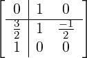 , y[n] = , y[n] = ![[ ]
y[n]
0[n]
y1](developer-guide48x.png) = = ![[ ]
m (tn,yn )
Δtl(tn-1,yn- 1)](developer-guide49x.png) |
![[ | ]
-A-|U---
B |V](developer-guide50x.png) = = 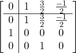 , y[n] = , y[n] = ![⌊ ⌋
y [n]
|| 0[n] ||
⌈ y 1 ⌉
y [n2]](developer-guide52x.png) = = 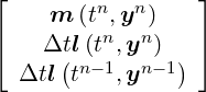 |
![[ | ]
AIM AEM |U
-BIM--BEM---|V--
|](developer-guide54x.png) = = ![⌊ [ 1 ] [ 0 ] |[ 1 1 ] ⌋
|-[---]--[---]-|[------]-|
|⌈ 1 0 | 1 1 |⌉
0 1 | 0 0](developer-guide55x.png) with y[n] = with y[n] = ![[ ]
y [n0]
[n]
y 1](developer-guide56x.png) = = ![[ ]
m (tn,yn)
Δtl (tn,yn )](developer-guide57x.png) |
![[ IM EM | ]
-A-IM---A-EM-|U--
B B |V](developer-guide58x.png) = = ![⌊ [ ] [ ] | [ ] ⌋
|-⌊--23-⌋--⌊-0-⌋-|⌊--43----13--43----23-⌋-|
|| 2 0 | 4 - 1 4 - 2 ||
|| || 30 || || 0 || ||| 31 03 30 03 || ||
|⌈ |⌈ |⌉ |⌈ |⌉ ||⌈ |⌉ |⌉
0 1 | 0 0 0 0
0 0 0 0 1 0](developer-guide59x.png) |
with
y[n] = ![⌊ y[n]⌋
| 0[n]|
|| y1 ||
|⌈ y[2n]|⌉
y[n]
3](developer-guide60x.png) = = 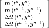 |
![[ | ]
-AIM---AEM---U--
BIM BEM |V
|](developer-guide62x.png) = = ![[ ] [ ] | [ ]
⌊ 6- 0 | 18- - -9 -2 18 - 18 6- ⌋
|-⌊--161-⌋--⌊---⌋-|⌊--1118----119--112--1118----1118--161-⌋-|
|| 11 0 | 11 - 11 11 11 - 11 11 ||
|| || 0 || || 0 || ||| 1 0 0 0 0 0 || ||
|| || 0 || || 0 || ||| 0 1 0 0 0 0 || ||
|| || 0 || || 1 || ||| 0 0 0 0 0 0 || ||
|⌈ |⌈ 0 |⌉ |⌈ 0 |⌉ ||⌈ 0 0 0 1 0 0 |⌉ |⌉
0 0 | 0 0 0 0 1 0](developer-guide63x.png) |
with
y[n] = ![⌊ y[n]⌋
|| 0[n]||
|| y1 ||
|| y[2n]||
|| y[n]||
|| 3[n]||
⌈ y4 ⌉
y[5n]](developer-guide64x.png) = = 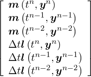 |
![[ | ]
-A-|U---
B |V](developer-guide66x.png) = = 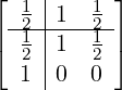 , y[n] = , y[n] = ![[ [n]]
y0
y[1n]](developer-guide68x.png) = = ![[ ]
m (tn,yn)
Δtl (tn,yn )](developer-guide69x.png) |
![[ | ]
-A--|U--
B |V](developer-guide70x.png) = = 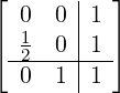 , y[n] = , y[n] = ![[ [n] ]
y 0](developer-guide72x.png) = = ![[ n n ]
m (t ,y )](developer-guide73x.png) |
![[ ]
A |U
-B--|V--
|](developer-guide74x.png) = = 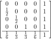 , y[n] = , y[n] = ![[ ]
y[n0]](developer-guide76x.png) = = ![[ ]
m (tn,yn)](developer-guide77x.png) |
![[ | ]
-A-|U---
B |V](developer-guide78x.png) = = 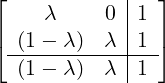 with λ = with λ =  , y[n] = , y[n] = ![[ ]
[n]
y0](developer-guide81x.png) = = ![[ ]
m (tn,yn )](developer-guide82x.png) |
![[ | ]
-A--|U--
B |V](developer-guide83x.png) = = 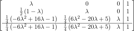 |
with
λ = 0.4358665215, y[n] = ![[ [n] ]
y 0](developer-guide85x.png) = = ![[ n n ]
m (t ,y )](developer-guide86x.png) |
![[ AIM AEM |U ]
-BIM--BEM-|V--](developer-guide87x.png) = = | |||
![⌊ ⌊ 0 0 0 0⌋ [ 0 0 0 0 ] |[ 1 ] ⌋
| ⌈ 00 1(1λ- λ) 0λ 00⌉ λ 0 0 0 | 1 |
|⌈ 0 14(-62λ2+16λ- 1) 14 (6λ2- 20λ+ 5) λ 0-.302.11207588588862906 00.3.5965269524937144779 0.55209291479 00 | 11 |⌉
-[-0--1(-6λ2+16λ--1)--1-(6λ2--20λ+-5)--λ ]--[-0-1-(--6λ2+-16λ-- 1)-1(6λ2- 20λ+-5)-λ-]-|[-1-]--
4 4 4 4 |](developer-guide88x.png) |
with
λ = 0.4358665215, y[n] = ![[ ]
y [n]
0](developer-guide89x.png) = = ![[ ]
m (tn,yn)](developer-guide90x.png) |
![[ ]
A |U
-B--|V--
|](developer-guide91x.png) = = ![[ ]
0 | 1
-φ-(z)-|φ-(z)-
0 | 0](developer-guide92x.png) , y[n] = , y[n] = ![[ ]
y [n0]](developer-guide93x.png) = = ![[ ]
m (tn,yn)](developer-guide94x.png) |
![[ A |U ]
----|---
B |V](developer-guide95x.png) = = ![[ 0 | 1 ]
-------|------
φ1(z) |φ0(z)](developer-guide96x.png) , y[n] = , y[n] = ![[ ]
y [n0]](developer-guide97x.png) = = ![[ ]
m (tn,yn)](developer-guide98x.png) |