|
Nektar++
|


All Classes Namespaces Files Functions Variables Typedefs Enumerations Enumerator Friends Macros Pages
|
Nektar++
|
Here, we will explain how to use the incompressible Navier-Stokes solver of Nektar++ using the direct solver. Its source code is located at Nektar++/solvers/IncNavierStokesSolver/EquationSystems. We will start by showing the formulation and demonstrating how to run a first example with the incompressible Navier-Stokes solver and briefly explain the options of the solver specified in the input file. After these introductory explanations, we will present some numerical results in order to demonstrate the capabilities and the accuracy of the solver.
We consider the weak form of the Stokes problem for the velocity field ![$\boldsymbol{v}=[u,v]^{T}$](form_0.png) and the pressure field
and the pressure field  :
:
![\[ (\nabla \phi,\nu \nabla \boldsymbol{v}) - (\nabla\cdot\phi,p)=(\phi,\boldsymbol{f}) \]](form_2.png)
![\[ (q,\nabla \cdot \boldsymbol{v}) = 0 \]](form_3.png)
where  ,
,  and
and  are appropriate spaces for the velocity and the pressure system to satisfy the inf-sup condition. Using a matrix notation the discrete system may be written as:
![\begin{displaymath} \left[ \begin{array}{ccc} A & D_b^T & B\\ D_b & 0 & D_i^T\\ B^T & D_i & C \end{array}\right] \left[ \begin{array}{c} \boldsymbol{v_b}\\ p\\ \boldsymbol{v_i} \end{array}\right] = \left[ \begin{array}{c} \boldsymbol{f_b}\\ 0\\ \boldsymbol{f_i} \end{array}\right] \end{displaymath}](form_7.png)
where the components of  and
and  are
are  ,
,  and
and  and the components
  and
and  are
are  and
and  . The indices
  and
and  refer to the degrees of freedom on the elemental boundary and interior, respectively. In constructing the system we have lumped the contributions form each component of the velocity field into matrices and . However we note that for a Newtonian fluid the contribution from each field is decoupled. Since the inetrior degrees of freedom of the velocity field do not overlap, the matrix is block diagonal and to take advantage of this structure we can statically condense out the matrix to obtain the system:
![\begin{displaymath} \left[ \begin{array}{ccc} A-BC^{-1}B^T & D_b^T-BC^{-1}D_i & 0\\ D_b-D_i^TC^{-1}B^T & -D_i^TC^{-1}D_i & 0\\ B^T & D_i & C \end{array}\right] \left[ \begin{array}{c} \boldsymbol{v_b}\\ p\\ \boldsymbol{v_i} \end{array}\right] = \left[ \begin{array}{c} \boldsymbol{f_b} - BC^{-1}\boldsymbol{f_i}\\ -D_i^TC^{-1}\boldsymbol{f_i}\\ \boldsymbol{f_i} \end{array}\right] \end{displaymath}](form_19.png)
To extend the aboce Stokes solver to an unsteady Navier-Stokes solver we first introduce the unsteady term,  , into the Stokes problem. This has the principal effect of modifying the weak Laplacian operator
  into a weak Helmholts operator
  where
where  depends on the time integration scheme. The second modification requires the explicit discretisation of the non-linear terms in a similar manner to the splitting scheme and this term is then introduced as the forcing term
  .
.
The folder Nektar++/regressionTests/Solvers/IncNavierStokesSolver/InputFiles contains several *.xml files. These are input files for the Navier-Stokes solver specifying the geometry (i.e. the mesh and the spectal/hp expansion), the parameters and boundary conditions. Further details on the structure of the input file can be found in pageXML.
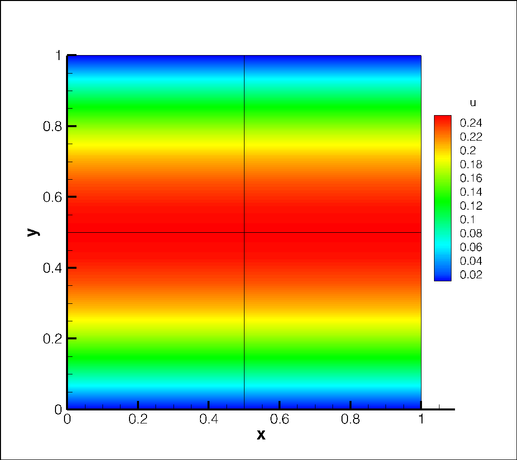
Now, lets try to run one of them with the coupled solver.
Test_ChanFlow_LinNS_m8.xml to the directory where the solver is compiled, e.g. Nektar++/solvers/IncNavierStokesSolver/build/IncNavierStokesSolver.The solution should now have been written to the file Test_ChanFlow_LinNS_m8.fld. This file is formatted in the Nektar++ output format. To visualise the solution, we can convert the fld-file into TecPlot, Gmsh or Tecplot file formats using the Post-processing tools in Nektar++/utilities/builds/PostProcessing/. Here, we will demonstrate how to convert the fld-file into TecPlot-file format.
We convert the fld-file into Tecplot-file format by typing
It will create Test_ChanFlow_LinNS_m8.dat which can be loaed in TecPlot.
A detailed descriptions of the input file for Nektar++ can be found in pageXML. For what concern the incompressible Navier-Stokes solver a typical set is:
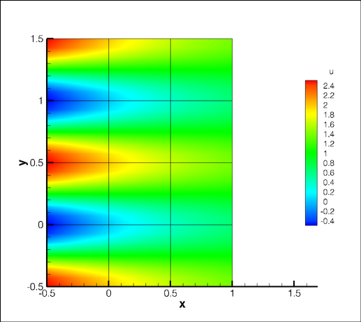
Futher options can be specified in the input file, as for the Steady Oseen Flow:
[1] S.J. Sherwin and M. Ainsworth: Unsteady Navier-Stokes Solvers Using Hybrid Spectral/hp Element Methods, Conference Paper, 2000.
[2] R. Stenberg and M. Suri: Mixed hp finite element methods for problems in elasticity and Stokes flows, Numer. Math, 72, 367-389, 1996.
[3] M. Ainsworth and S.J. Sherwin: Domain decomposition preconditioners for p and hp finite element approximation of the Stokes equations, Comput. Methods Appl. Mech. Engrg., 175, 243-266, 1999.
[4] P. La Tallec and A. Patra: Non-overlapping domain decomposition methods for adaptive hp approximations of the Stokes problem with discontiunous pressure field, Comput. Methods Appl. Mech. Engrg., 145, 361-379, 1997.
[5] G. E. Karniadakis, M. Israeli, and S. A. Orszag: High-order splitting methodsfor the incompressible Navier-Stokes equations, J. Comput. Phys., 97, 414-443, 1991.
 1.8.8
1.8.8