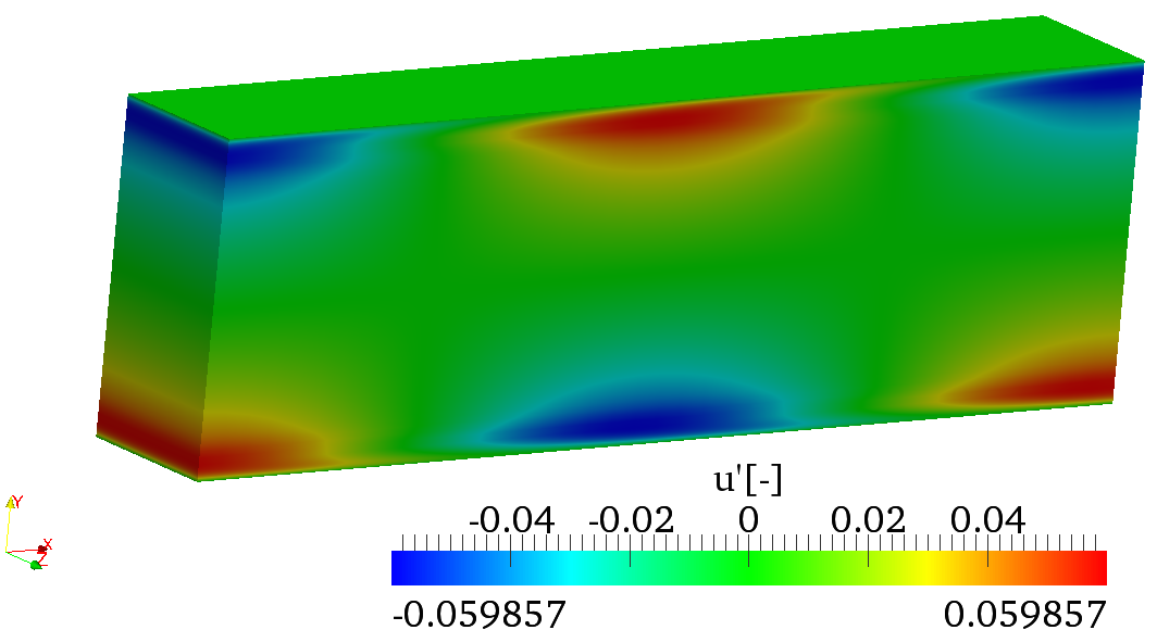
(a)
u′ |
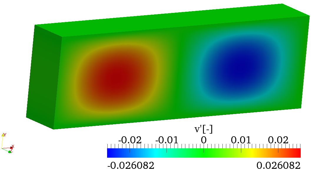
(b)
v′ |
Figure 14: u′- and v′-component of the eigenmode.
Now that we have presented the various stability-analysis tools present in Nektar++ , we conclude showing
the capabilities of the code in three spatial dimensions. In the folder $NEKTUTORIAL/Channel-3D/Stability there are the files that are required for the stability analysis - note
that we do not show the geometry and the base flow generation (we will be using the exact solution) since
we have already presented these features in the previous tutorials.
The case considered is similar to the channel flow presented in section 1. However, in this case the Reynolds number is set to 10000. In order to run a three-dimensional simulation, we can either run the full 3D solver by creating a 3D geometry or use a 2D geometry and specify the use of a Fourier expansion in the third direction. The last method is also known as 3D homogenous 1D approach. Here we will present this approach.
Specifically, we use a 2D geometry and we add the various parameters necessary to use the
Fourier expansion. Note that in the 2D plane we will use a MODIFIED expansion basis with
NUMMODES=11.
$NEKTUTORIAL/Channel-3D/Stability/PPF_R10000_3D.xml, make the following
changes:
SOLVERINFO tag called HOMOGENEOUS and set it to 1D.
SOLVERINFO tags called ModeType and BetaZero and set them to
SingleMode and True, respectively.
PARAMETERS called HomModesZ and LZ and set them to 2 and 1, respectively.
PARAMETERS called realShift and imagShift and set them to 0.003 and
0.2, respectively.Now run the solver - the terminal screen should look like this:
Now convert the two files containing the eigenvectors and visualise them in Paraview or VisIt - the solution should look like the one below:
$NEKTUTORIAL/Channel-3D/Stability/PPF_R15000_3D.xml has been
provided to show a full 3D unstable eigenmode where β is not zero. Run this file and see that
you obtain the eigenvalue 0.00248682 ±−0.158348i