After having computed the base flow it is now possible to calculate the eigenvalues and the eigenmodes of the linearised Navier-Stokes equations. Two different algorithms can be used to solve the equations:
VelocityCorrectionScheme) and
CoupledLinearisedNS).We will consider both cases, highlighting the similarities and differences of these two methods. In this tutorial we will use the Implicitly Restarted Arnoldi Method (IRAM), which is implemented in the open-source library ARPACK and the modified Arnoldi algorithm1 that is also available in Nektar++.
First, we will compute the leading eigenvalues and eigenvectors using the velocity
correction scheme method. In the $NEKTUTORIAL/stability folder there is a file called
Channel-VCS.xml. This file is similar to Channel-Base.xml, but contains additional
instructions to perform the direct stability analysis.
Note: The entire GEOMETRY section, and EXPANSIONS section must be identical to that used to
compute the base flow.
SOLVERINFO options which are related to the
stability analysis.
EvolutionOperator to Direct in order to activate the forward linearised
Navier-Stokes system.
Driver to Arpack in order to use the ARPACK eigenvalue analysis.
ArpackProblemType. In particular, set ArpackProblemType to LargestMag to get
the eigenvalues with the largest magnitude (that determines the stability of the
flow).
Note: It is also possible to select the eigenvalue with the largest real part by
setting ArpackProblemType to (LargestReal) or with the largest imaginary part
by setting ArpackProblemType to (LargestImag).
kdim=16: dimension of Krylov-space,
nvec=2: number of requested eigenvalues,
nits=500: number of maximum allowed iterations,
evtol=1e-6: accepted tolerance on the eigenvalues and it determines the stopping
criterion of the method.FUNCTION called InitialConditions and BaseFlow.
InitialConditions function to be read from
Channel-VCS.rst. The solution will then converge after 16 iterations after it has
populated the Krylov subspace.
Note: The restart file is a field file (same format as .fld files) that contains the
eigenmode of the system.
Note: Since the simulations often take hundreds of iterations to converge, we
will not initialise the IRAM method with a random vector during this tutorial.
Normally, a random vector would be used by setting the SolverInfo option
InitialVector to Random.
Channel-Base.fld), computed in the previous section, should
be copied into the Channel/Stability folder and renamed Channel-VCS.bse.
Now specify a function called BaseFlow which reads this file.$NEK/IncNavierStokesSolver Channel-VCS.xml
At the end of the simulation, the terminal screen should look like this:
The eigenvalues are computed in the exponential form Meiθ where M = |λ| is the magnitude, while θ = arctan(λi∕λr) is the phase:
|
| (3.1) |
It is interesting to consider more general quantities that do not depend on the time length chosen for each iteration T. For this purpose we consider the growth rate σ = ln(M)∕T and the frequency ω = θ∕T.
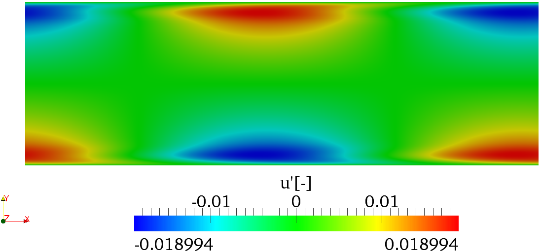
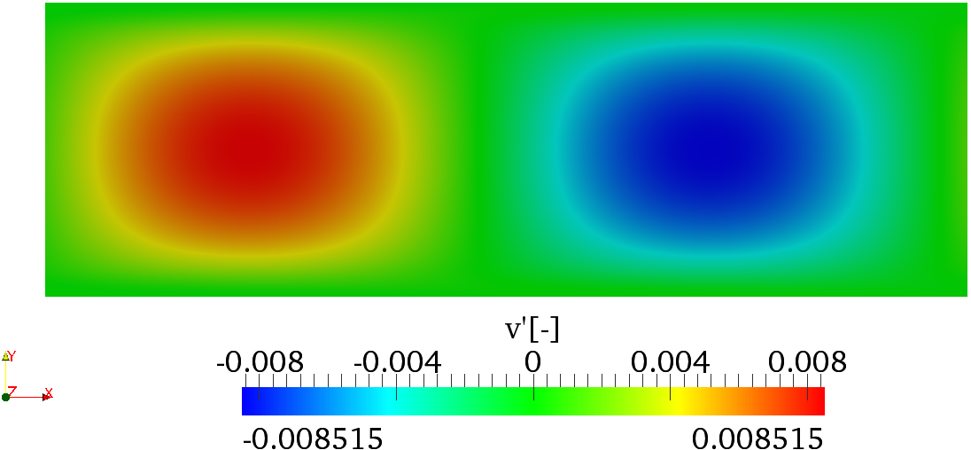
Figure 3.1 shows the profile of the computed eigenmode. The eigenmodes associated
with the computed eigenvalues are stored in the files Channel_VCS_eig_0.fld and
Channel_VCS_eig_1.fld. It is possible to convert this file into VTK format in the same way
as previously done for the base flow.
| σ | = 2.2353 × 10⁻³ | ||
| ω | = ±2.49892 × 10⁻¹ |
and that the eigenmodes match those given in figures 3.1.
Driver to ModifiedArnoldi. You can
now try to re-run the simulation and verify that the modified Arnoldi algorithm
provides a results that is consistent with the previous computation obtained with
Arpack.
Note: Remember to use the files provided in the folder Stability/Coupled for this
case.
It is possible to perform the same stability analysis using a different method based on the Coupled Linearised Navier-Stokes algorithm. This method requires the solution of the full velocity-pressure system, meaning that the velocity matrix system and the pressure system are coupled, in contrast to the velocity correction scheme/splitting schemes.
Inside the folder $NEKTUTORIAL/stability there is a file called Channel-Coupled.xml that
contains all the necessary parameters that should be defined. In this case we will specify the
base flow through an analytical expression. Even in this case, the geometry, the type and
number of modes are the the same of the previous simulations.
Channel-Coupled.xml:
Note: As before the bits to be completed are identified by …in this file.
SolverType property to CoupledLinearisedNS in order to solve the
linearised Navier-Stokes equations using Nektar + +’s coupled solver.
EQTYPE must be set to SteadyLinearisedNS and the Driver to Arpack.
InitialVector property to Random to initialise the IRAM with a random
initial vector. In this case the function InitialConditions will be ignored.
LargestMag in the
property ArpackProblemType.It is important to note that the use of the coupled solver requires that only the velocity component variables are specified, while the pressure is implicitly evaluated.
Channel-Coupled.xml:
SteadyLinearisedNS coupled solver,
this is defined through a function called AdvectionVelocity. The u component
must be set up to 1 - y2, while the v-component to zero.CONDITIONS tag:
This has already been set up in the XML file. This is necessary to tell Nektar++ to use the previous solution as the right hand side vector for each Arnoldi iteration.
$NEK/IncNavierStokesSolver Channel-Coupled.xml
The terminal screen should look like this:
Using the Stokes algorithm, we are computing the leading eigenvalue of the inverse of the operator L-1. Therefore the eigenvalues of L are the inverse of the computed values2 . However, it is interesting to note that these values are different from those calculated with the Velocity Correction Scheme, producing an apparent inconsistency. However, this can be explained considering that the largest eigenvalues associated to the operator L correspond to the ones that are clustered near the origin of the complex plane if we consider the spectrum of L-1. Therefore, eigenvalues with a smaller magnitude may be present but are not associated with the largest-magnitude eigenvalue of operator L. One solution is to consider a large Krylov dimension specified by kdim and the number of eigenvalues to test using nvec. This will however take more iterations. Another alternative is to use shifting but in this case it will make a real problem into a complex one (we shall show an example later). Finally, another alternative is to search for the eigenvalue with a different criterion, for example, the largest imaginary part.
ArpackProblemType to LargestImag and run the
simulation again.
In this case, it is easy to to see that the eigenvalues of the evolution operator L are the same ones computed in the previous section with the time-stepping approach (apart from round-off errors). It is interesting to note that this method converges much quicker that the time-stepping algorithm. However, building the coupled matrix that allows us to solve the problem can take a non-negligible computational time for more complex cases.
Now that we have presented the various stability-analysis tools present in Nektar++, we
conclude showing the capabilities of the code in three spatial dimensions. In the folder
$NEKTUTORIAL/stability3D there are the files that are required for the stability analysis -
note that we do not show the geometry and the base flow generation (we will be using
the exact solution) since we have already presented these features in the previous
tutorials.
The case considered is similar to the channel flow presented in section 2. However, in this case the Reynolds number is set to 10000. In order to run a three-dimensional simulation, we can either run the full 3D solver by creating a 3D geometry or use a 2D geometry and specify the use of a Fourier expansion in the third direction. The last method is also known as 3D homogenous 1D approach. Here we will present this approach.
Specifically, we use a 2D geometry and we add the various parameters necessary to use the
Fourier expansion. Note that in the 2D plane we will use a MODIFIED expansion basis with
NUMMODES=11.
$NEKTUTORIAL/stability3D/PPF_R10000_3D.xml, make the following
changes:
SOLVERINFO tag called HOMOGENEOUS and set it to 1D.
SOLVERINFO tags called ModeType and BetaZero and set them
to SingleMode and True, respectively.
PARAMETERS called HomModesZ and LZ and set them to 2 and 1,
respectively.
PARAMETERS called realShift and imagShift and set them to
0.003 and 0.2, respectively.Now run the solver - the terminal screen should look like this:
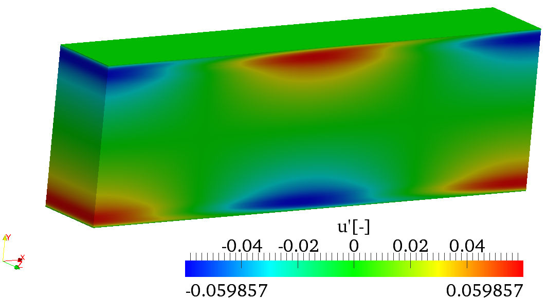
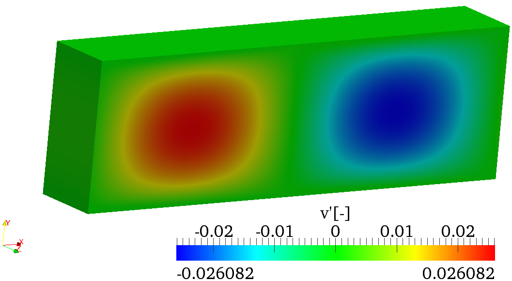
Now convert the two files containing the eigenvectors and visualise them in Paraview or VisIt - the solution should look like the one below:
$NEKTUTORIAL/stability3D/PPF_R15000_3D.xml has
been provided to show a full 3D unstable eigenmode where β is not zero. Run this file and see
that you obtain the eigenvalue 0.00248682 ±-0.158348i
Completed solutions to the tutorials are available in the completed directory.
This completes the tutorial.