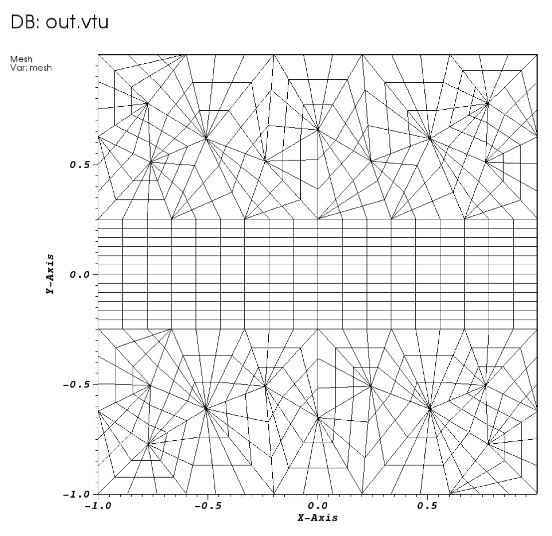
Figure 2.1: Mesh generated by Gmsh.
As already mentioned to set up the problem we have two step. The first is setting up a mesh in an input xml format consistent with Nektar++ as discussed in section 2.1. We also need to configure the problem initial, boundary and parameters which are discussed in 2.2.
The first pre-processing step consists in generating the mesh in a Nektar++ compatible format. One option to do this is to use the open-source mesh-generator Gmsh to first create the geometry, that in our case is a square and successively the mesh. The mesh format provided by Gmsh shown in Fig. (2.1) - i.e. .msh extension - is not consistent with the Nektar++ solvers and, therefore, it needs to be converted.
To do so, we need to run the pre-processing routine called NekMesh within Nektar++. This
routine requires two line arguments, the mesh file generated by Gmsh, ADR_mesh.msh, and the
name of the Nektar++-compatible mesh file that NekMesh will generate, for instance
ADR_mesh.xml. The command line for this step is
$NEK/NekMesh ADR_mesh.msh ADR_mesh.xml
or
$NEK/NekMesh ADR_mesh.msh ADR_mesh.xml:xml:uncompress
NekMesh to write the file
out in uncompressed format. The generated .xml mesh file is reported below and can also
be found in the completed directory. It contains 5 tags encapsulated within the
GEOMETRY tag, which describes the mesh. The first tag, VERTEX, contains the spatial
coordinates of the vertices of the various elements of the mesh. The second tag,
EDGE contains the lines connecting the vertices. The third tag, ELEMENT, defines the
elements (note that in this case we have both triangular - e.g. <T ID="0"> - as
well as quadrilateral - e.g. <Q ID="85"> - elements). The fourth tag, COMPOSITE, is
constituted by the physical regions of the mesh called composite, where the composites
formed by elements represent the solution sub-domains - i.e. the mesh sub-domains
where we want to solve the linear advection problem (note that we will use these
composites to define expansion bases on each sub-domain in section 2.2) - while the
composites formed by edges are the boundaries of the domain where we need to apply
suitable boundary conditions (note that we will use these composites to specify
the boundary conditions in section 2.2). Finally, the fifth tag, DOMAIN, formally
specifies the overall solution domain as the union of the three composites forming
the three solution subdomains (note that the specification of three subdomain -
i.e. composites - in this case is necessary since they are constituted by different
element shapes). For additional details on the GEOMETRY tag refer to the User-Guide.
1<?xml version="1.0" encoding="utf-8" ?>
2<NEKTAR>
3   <GEOMETRY DIM="2" SPACE="2">
4      <VERTEX>
5        <V ID="0">2.00000000e-01 -1.00000000e+00 0.00000000e+00</V>
6        <V ID="1">5.09667784e-01 -6.15240515e-01 0.00000000e+00</V>
7        ...
8        <V ID="68">-1.00000000e+00 1.25000000e-01 0.00000000e+00</V>
9      </VERTEX>
10      <EDGE>
11        <E ID="0"> 0 1 </E>
12        <E ID="1"> 1 2 </E>
13        ...
14        <E ID="153"> 40 68 </E>
15      </EDGE>
16      <ELEMENT>
17        <T ID="0"> 0 1 2 </T>
18        <T ID="1"> 3 4 5 </T>
19        ...
20        <Q ID="85"> 146 93 153 151 </Q>
21     </ELEMENT>
22      <COMPOSITE>
23        <C ID="1"> T[0-30] </C>
24        <C ID="2"> Q[62-85] </C>
25        <C ID="3"> T[31-61] </C>
26        <C ID="100"> E[46,12,20,10,45] </C>
27        <C ID="200"> E[50,32,108,111,114,117,87,103] </C>
28        <C ID="300"> E[100,64,74,66,99] </C>
29        <C ID="400"> E[49,33,148,150,152-153,86,104] </C>
30      </COMPOSITE>
31      <DOMAIN> C[1,2,3] </DOMAIN>
32   </GEOMETRY>
33</NEKTAR>
After having generated the mesh file in a Nektar++-compatible format, ADR_mesh.xml, we
can visualise the mesh. This step can be done by using the following Nektar++ built-in
post-processing routine:
$NEK/FieldConvert ADR_mesh.xml ADR_mesh.vtu
Alternatively a tecplot .dat file can be created by changing the extension of the second file, i.e.
$NEK/FieldConvert ADR_mesh.xml ADR_mesh.dat
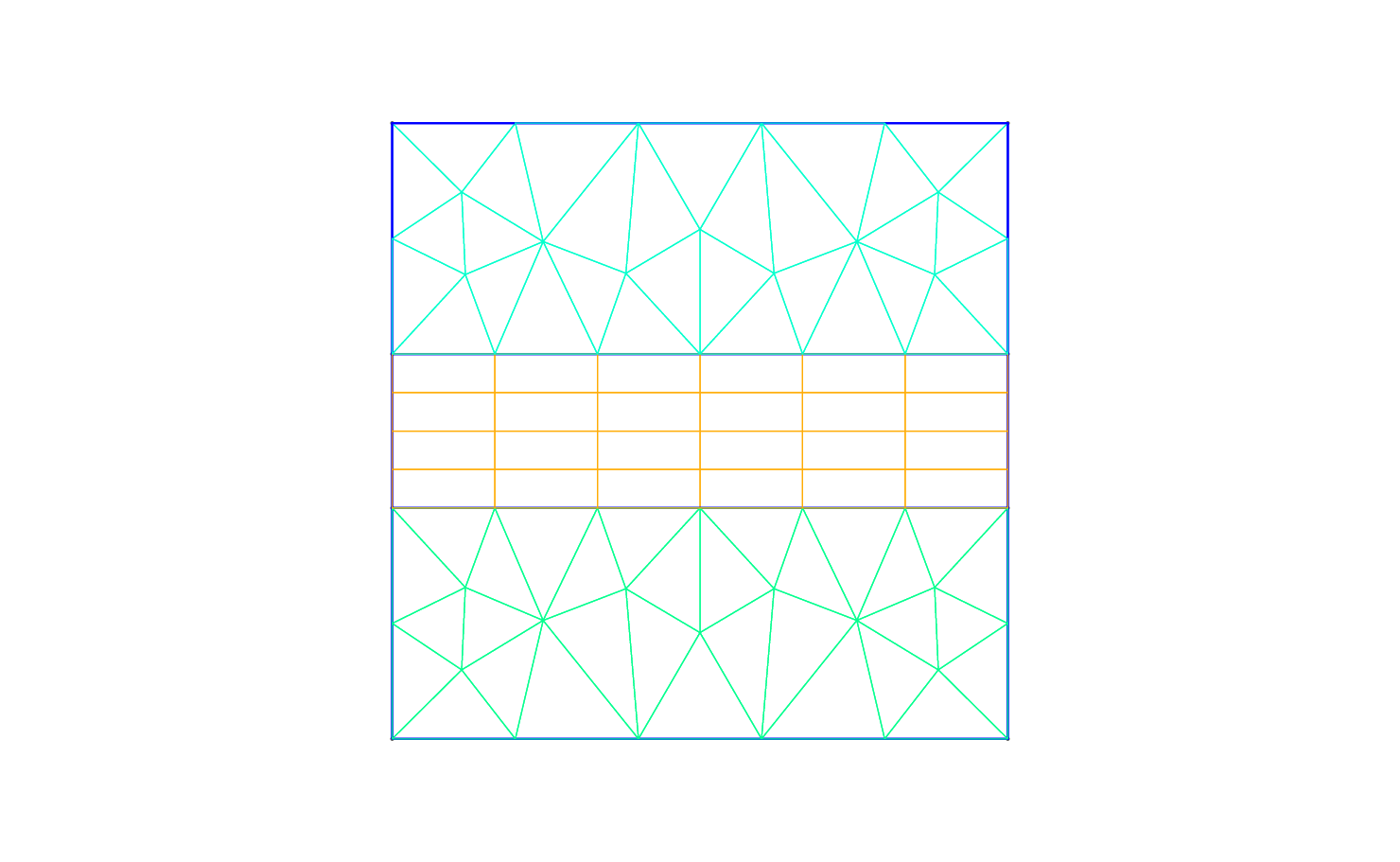
ADR_mesh.vtu file which can be directly read by the open-source
visualisation tool called Paraview or VisIt. In Fig. 2.2 we show the mesh distribution for the
mesh considered in this tutorial, ADR_mesh.xml. Before configuring the input files, if we want to use periodic boundary conditions, we need to
make sure that the edges of the two periodic boundaries (i.e. xb = [-1,1],yb) are properly
aligned. Gmsh and the NekMesh routine within Nektar++ does not guarantee proper
alignment. However, NekMesh provides a module, called peralign, that enforces the reordering
of pair of edges (for more details refer to the User-Guide. We can apply this by using the
following command:
$NEK/NekMesh -m peralign:surf1=200:surf2=400:dir=x ADR_mesh.xml
 ADR_mesh_aligned.xml
-m peralign is selecting the module for aligning the edges which are specified by surf1
and surf2 (their IDs in this case are 200 and 400) and dir is the direction to which the two
periodic edges are perpendicular (in this case x). Note that since we have not used the
extension :xml:uncompress the blocks of data in this file are now stored in compressed
format.
After having typed the last command, we have a mesh, ADR_mesh_aligned.xml, which is fully
compatible with Nektar++ and which allows us applying periodic boundary conditions
without encountering errors.
We can therefore now configure the conditions: initial conditions, boundary conditions, parameters and solver settings.
To set the various problem parameters, the solver settings, initial and boundary conditions
and the expansion basese, we use the file called ADR_conditions.xml, which can
be found within the tutorial directory for this tutorial. This new file contains
the CONDITIONS tag where we can specify the parameters of the simulations, the
solver settings, the initial conditions, the boundary conditions and the exact solution
and contains the EXPANSIONS tag where we can specify the polynomial order to be
used inside each element of the mesh, the type of expansion bases and the type of
points.
We begin to describe the ADR_conditions.xml file from the CONDITIONS tag, and in
particular from the boundary conditions, initial conditions and exact solution sections:
1<CONDITIONS>
2   ...
3   ...
4   ...
5   <VARIABLES>
6      <V ID="0"> u </V>
7   </VARIABLES>
8
9   <BOUNDARYREGIONS>
10      <B ID="0"> C[100] </B>
11      <B ID="1"> C[200] </B>
12      <B ID="2"> C[300] </B>
13      <B ID="3"> C[400] </B>
14   </BOUNDARYREGIONS>
15
16   <BOUNDARYCONDITIONS>
17      <REGION REF="0">
18        <D VAR="u" USERDEFINEDTYPE="TimeDependent"
19        VALUE="sin(k*(x-advx*t))*cos(k*(y-advy*t))" />
20      </REGION>
21      <REGION REF="1">
22        <P VAR="u" VALUE="[3]" />
23      </REGION>
24      <REGION REF="2">
25         <D VAR="u" USERDEFINEDTYPE="TimeDependent"
26        VALUE="sin(k*(x-advx*t))*cos(k*(y-advy*t))" />
27      </REGION>
28      <REGION REF="3">
29        <P VAR="u" VALUE="[1]" />
30      </REGION>
31   </BOUNDARYCONDITIONS>
32
33   <FUNCTION NAME="InitialConditions">
34      <E VAR="u" VALUE="sin(k*x)*cos(k*y)" />
35   </FUNCTION>
36
37   <FUNCTION NAME="AdvectionVelocity">
38      <E VAR="Vx" VALUE="advx" />
39      <E VAR="Vy" VALUE="advy" />
40   </FUNCTION>
41
42   <FUNCTION NAME="ExactSolution">
43      <E VAR="u" VALUE="sin(k*(x-advx*t))*cos(k*(y-advy*t))" />
44   </FUNCTION>
45</CONDITIONS>
In the above piece of .xml, we first need to specify the non-optional tag called VARIABLES that
sets the solution variable (in this case u).
The second tag that needs to be specified is BOUNDARYREGIONS through which the user can
specify the regions where to apply the boundary conditions. For instance, <B ID="0"> C[100]
</B> indicates that composite 100 (which has been introduced in section 2.1) has a boundary
ID equal to 0. This boundary ID is successively used to prescribe the boundary
conditions.
The third tag is BOUNDARYCONDITIONS by which the boundary conditions are actually specified
for each boundary ID specified in the BOUNDARYREGIONS tag. The syntax <D VAR="u"
corresponds to a Dirichlet boundary condition for the variable u (note that in this case we used
the additional tag USERDEFINEDTYPE="TimeDependent" which is a special option when using
time-dependent boundary conditions), while <P VAR="u" corresponds to Periodic boundary
conditions. For additional details on the various options possible in terms of boundary
conditions refer to the User-Guide.
Finally, <FUNCTION NAME="InitialConditions"> allows the specification of the initial
conditions, <FUNCTION NAME="AdvectionVelocity"> specifies the advection velocities in
both the x- and y-direction (for this two-dimensional case) and is a non-optional
parameters for the unsteady advection equation and <FUNCTION NAME="ExactSolution">
permits us to provide the exact solution, against which the L2 and L∞ errors are
computed.
After having configured the VARIABLES tag, the initial and boundary conditions, the advection
velocity and the exact solution we can complete the tag CONDITIONS prescribing the
parameters necessary (PARAMETERS), solver settings (SOLVERINFO), and time integration
scheme (TIMEINTEGRATIONSCHEME):
1<CONDITIONS>
2   <PARAMETERS>
3      <P> FinTime = 1.0 </P>
4      <P> TimeStep = 0.001 </P>
5      <P> NumSteps = FinTime/TimeStep </P>
6      <P> IO_InfoSteps = 100 </P>
7      <P> advx = 2.0 </P>
8      <P> advy = 0.0 </P>
9      <P> k = 2*PI </P>
10   </PARAMETERS>
11
12   <SOLVERINFO>
13      <I PROPERTY="EQTYPE" VALUE="UnsteadyAdvection" />
14      <I PROPERTY="Projection" VALUE="DisContinuous" />
15      <I PROPERTY="AdvectionType" VALUE="WeakDG" />
16      <I PROPERTY="UpwindType" VALUE="Upwind" />
17   </SOLVERINFO>
18
19   <TIMEINTEGRATIONSCHEME>
20      <METHOD> RungeKutta </METHOD>
21      <ORDER> 4 </ORDER>
22   </TIMEINTEGRATIONSCHEME>
23   ...
24   ...
25   ...
In the PARAMETERS tag, FinTime is the final physical time of the simulation, TimeStep is the
time-step, NumSteps is the number of steps, IO_InfoSteps is the step-interval when some
information about the simulation are printed to the screen, advx and advy are the advection
velocities Vx and Vy, respectively and k is the κ parameter. Note that advx, advy and k are
used in the boundary and initial conditions tags as well as in the specification of the advection
velocities. To output periodic checkpoint files every 100 time steps, a Checkpoint filter is
applied:
1<FILTERS>
2 <FILTER TYPE="Checkpoint">
3   <PARAM NAME="OutputFrequency">100</PARAM>
4 </FILTER>
5</FILTERS>
In the SOLVERINFO tag, EQTYPE is the type of equation to be solved, Projection is the spatial
projection operator to be used (which in this case is specified to be ‘DisContinuous’),
AdvectionType is the advection operator to be adopted (where the VALUE ‘WeakDG’ implies
the use of a weak Discontinuous Galerkin technique), UpwindType is the numerical flux to be
used at the element interfaces when a discontinuous projection is used. For additional
solver-setting options refer to the User-Guide.
Finally, we need to specify the expansion bases we want to use in each of the three composites
or sub-domains (COMPOSITE="..") introduced in section 2.1:
1<EXPANSIONS>
2   <E COMPOSITE="C[1]" NUMMODES="5" TYPE="MODIFIED" FIELDS="u" />
3   <E COMPOSITE="C[2]" NUMMODES="5" TYPE="MODIFIED" FIELDS="u" />
4   <E COMPOSITE="C[3]" NUMMODES="5" TYPE="MODIFIED" FIELDS="u" />
5</EXPANSIONS>
In particular, for all the composites, COMPOSITE="C[i]" with i=1,2,3 we select identical basis
functions and polynomial order, where NUMMODES is the number of coefficients we want to use
for the basis functions (that is commonly equal to P+1 where P is the polynomial order of the
basis functions), TYPE allows selecting the basis functions FIELDS is the solution variable of
our problem and COMPOSITE are the mesh regions created by Gmsh. For additional details on
the EXPANSIONS tag refer to the User-Guide.
ADR_conditions.xml or copy it from the completed
directory.