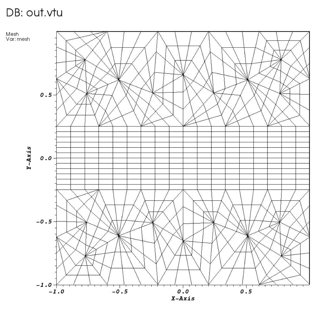
Figure 2.1: Mesh generated by Gmsh.
The pre-processing step consists of generating the mesh in a Nektar++ compatible format. To do this we can use the open-source mesh generator Gmsh to first define the geometry, which in our case is a square mesh. The resulting mesh is shown in Fig. 2.1. The mesh file format (.msh) generated by Gmsh is not directly compatible with the Nektar++ solvers and, therefore, it needs to be converted.
To do so, we need to run the Nektar++ pre-processing routine called NekMesh. This routine
requires two command-line arguments: the mesh file generated by Gmsh, Helm_mesh.msh; and
the name of the Nektar++-compatible mesh file that NekMesh will generate, for instance
Helm_mesh.xml.
$NEKTUTORIAL directory by calling
$NEK/NekMesh Helm_mesh.msh Helm_mesh.xml
or
$NEK/NekMesh Helm_mesh.msh Helm_mesh.xml:xml:uncompress
NekMesh to write the
file out in uncompressed ASCII format. The generated .xml mesh file is shown below and can
also be found in the completed directory. It contains 5 tags encapsulated within the GEOMETRY
tag, which describes the mesh. The first tag, VERTEX, contains the spatial coordinates of the
vertices of the various elements of the mesh. The second tag, EDGE contains the lines
connecting the vertices. The third tag, ELEMENT, defines the elements (note that in this
case we have both triangular - e.g. <T ID="0"> - as well as quadrilateral - e.g. <Q
ID="85"> - elements). The fourth tag, COMPOSITE, describes the physical regions of the
mesh and each composite may contain only one type of mesh entity. There are three
composites composed of triangular or quadrilateral elements which represent the
solution sub-domains where we want to solve the linear advection problem. We will
use these composites to define expansion bases on each sub-domain in section 2.1.
The composites formed by edges are the boundaries of the domain where we will
prescribe suitable boundary conditions in section 2.1. Finally, the fifth tag, DOMAIN,
formally specifies the overall solution domain as the union of the three element
composites. For additional details on the GEOMETRY specification refer to the User-Guide.
1<?xml version="1.0" encoding="utf-8" ?>
2<NEKTAR>
3   <GEOMETRY DIM="2" SPACE="2">
4      <VERTEX>
5        <V ID="0">2.00000000e-01 -1.00000000e+00 0.00000000e+00</V>
6        <V ID="1">5.09667784e-01 -6.15240515e-01 0.00000000e+00</V>
7        ...
8        <V ID="68">-1.00000000e+00 1.25000000e-01 0.00000000e+00</V>
9      </VERTEX>
10      <EDGE>
11        <E ID="0"> 0 1 </E>
12        <E ID="1"> 1 2 </E>
13        ...
14        <E ID="153"> 40 68 </E>
15      </EDGE>
16      <ELEMENT>
17        <T ID="0"> 0 1 2 </T>
18        <T ID="1"> 3 4 5 </T>
19        ...
20        <Q ID="85"> 146 93 153 151 </Q>
21     </ELEMENT>
22      <COMPOSITE>
23        <C ID="1"> T[0-30] </C>
24        <C ID="2"> Q[62-85] </C>
25        <C ID="3"> T[31-61] </C>
26        <C ID="100"> E[46,12,20,10,45] </C>
27        <C ID="200"> E[50,32,108,111,114,117,87,103] </C>
28        <C ID="300"> E[100,64,74,66,99] </C>
29        <C ID="400"> E[49,33,148,150,152-153,86,104] </C>
30      </COMPOSITE>
31      <DOMAIN> C[1,2,3] </DOMAIN>
32   </GEOMETRY>
33</NEKTAR>
After generating the mesh file in the Nektar++-compatible format, Helm_mesh.xml, we can
visualise the mesh. This step can be done by using the following Nektar++ built-in
post-processing routine:
$NEKTUTORIAL directory by calling
$NEK/FieldConvert Helm_mesh.xml Helm_mesh.vtu
Alternatively a tecplot .dat file can be created by changing the extension of the second file, i.e.
$NEK/FieldConvert Helm_mesh.xml Helm_mesh.dat
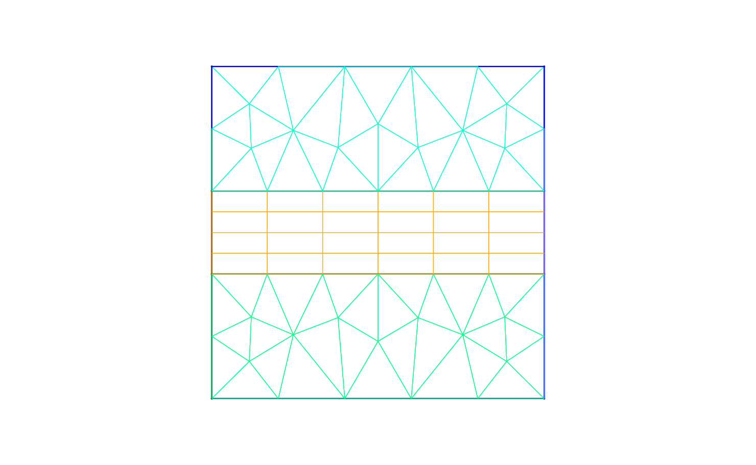
Helm_mesh.vtu file which can be directly read by the open-source
visualisation tool called Paraview or VisIt. In Fig. 2.2 we show the mesh distribution for the
mesh considered in this tutorial, Helm_mesh.xml. We can now configure the conditions: initial conditions, boundary conditions, parameters and solver settings.
To set the various parameters, the solver settings and the initial and boundary conditions
needed, we create a new file called Helm_conditions.xml, which can be found within the
completed directory for this tutorial. This new file contains the CONDITIONS tag where we can
specify the parameters of the simulations, the solver settings, the initial conditions, the
boundary conditions and the exact solution and contains the EXPANSIONS tag where we can
specify the polynomial order to be used inside each element of the mesh, the type of expansion
bases and the type of points.
We begin to describe the Helm_conditions.xml file from the CONDITIONS tag, and in
particular from the boundary conditions, initial conditions and exact solution sections:
1<CONDITIONS>
2   ...
3   ...
4   ...
5   <VARIABLES>
6      <V ID="0"> u </V>
7   </VARIABLES>
8
9   <BOUNDARYREGIONS>
10      <B ID="0"> C[100] </B>
11      <B ID="1"> C[200] </B>
12      <B ID="2"> C[300] </B>
13      <B ID="3"> C[400] </B>
14   </BOUNDARYREGIONS>
15
16   <BOUNDARYCONDITIONS>
17      <REGION REF="0">
18        <N VAR="u" VALUE="-PI*cos(PI*x)*sin(PI*y)" />
19      </REGION>
20      <REGION REF="1">
21        <D VAR="u" VALUE="cos(PI*x)*cos(PI*y)" />
22      </REGION>
23      <REGION REF="2">
24        <N VAR="u" VALUE="PI*cos(PI*x)*sin(PI*y)" />
25      </REGION>
26      <REGION REF="3">
27        <D VAR="u" VALUE="cos(PI*x)*cos(PI*y)" />
28      </REGION>
29   </BOUNDARYCONDITIONS>
30
31   <FUNCTION NAME="Forcing">
32      <E VAR="u" VALUE="-(Lambda␣+␣2*PI*PI)*cos(PI*x)*cos(PI*y)" />
33   </FUNCTION>
34
35   <FUNCTION NAME="ExactSolution">
36      <E VAR="u" VALUE="cos(PI*x)*cos(PI*y)" />
37   </FUNCTION>
38</CONDITIONS>
In the above piece of .xml, we first need to specify the non-optional tag called VARIABLES that
sets the solution variable (in this case u).
The second tag that needs to be specified is BOUNDARYREGIONS through which the user can
specify the regions where to apply the boundary conditions. For instance, <B ID="0"> C[100]
</B> indicates that composite 100 (which has been introduced in section 2) has a boundary
ID equal to 0. This boundary ID is successively used to prescribe the boundary
conditions.
The third tag is BOUNDARYCONDITIONS by which the boundary conditions are actually specified
for each boundary ID specified in the BOUNDARYREGIONS tag. The syntax <D VAR="u"
corresponds to a Dirichlet boundary condition for the variable u, while <N VAR="u"
corresponds to Neumann boundary conditions. For additional details on the various options
possible in terms of boundary conditions refer to the User-Guide.
Finally, <FUNCTION NAME="Forcing"> allows the specification of the Forcing function and
<FUNCTION NAME="ExactSolution"> permits us to provide the exact solution, against which
the L2 and L∞ errors are computed.
After having configured the VARIABLES tag, the boundary conditions, the forcing function and
the exact solution we can complete the tag CONDITIONS prescribing the parameters necessary
(PARAMETERS)and the solver settings (SOLVERINFO):
1<CONDITIONS>
2   <PARAMETERS>
3      <P> Lambda= 2.5 </P>
4   </PARAMETERS>
5
6   <SOLVERINFO>
7      <I PROPERTY="EQTYPE" VALUE="Helmholtz" />
8      <I PROPERTY="Projection" VALUE="Continuous" />
9   </SOLVERINFO>
10   ...
11   ...
12   ...
In the PARAMETERS tag, Lambda is the Helmholtz constant λ.
In the SOLVERINFO tag, EQTYPE is the type of equation to be solved, Projection is the spatial
projection operator to be used (which in this case is specified to be ‘Continuous’) For
additional solver-setting options refer to the User-Guide.
Finally, we need to specify the expansion bases we want to use in each of the three composites
or sub-domains (COMPOSITE="..") introduced in section 2:
1<EXPANSIONS>
2   <E COMPOSITE="C[1]" NUMMODES="5" TYPE="MODIFIED" FIELDS="u" />
3   <E COMPOSITE="C[2]" NUMMODES="5" TYPE="MODIFIED" FIELDS="u" />
4   <E COMPOSITE="C[3]" NUMMODES="5" TYPE="MODIFIED" FIELDS="u" />
5</EXPANSIONS>
In particular, for all the composites, COMPOSITE="C[i]" with i=1,2,3 we select identical basis
functions and polynomial order, where NUMMODES is the number of coefficients we want to use
for the basis functions (that is commonly equal to P+1 where P is the polynomial order of the
basis functions), TYPE allows selecting the basis functions FIELDS is the solution variable of
our problem and COMPOSITE are the mesh regions created by Gmsh. For additional details on
the EXPANSIONS tag refer to the User-Guide.
Helm_conditions.xml in the directory $NEKTUTORIAL with
λ = 2.5 or copy it from the completed directory.