Chapter 1
Introduction

The aim of this tutorial is to introduce the user to the spectral/hp element framework Nektar + + and to describe the main features of its Compressible Flow Solver in a simple manner. If you have not already downloaded and installed Nektar + +, please do so by visiting www.nektar.info, where you can also find the User-Guide with the instructions to install the library.

This tutorial requires:

• Nektar + + CompressibleFlowSolver and pre- and post-processing tools,

• The visualisation tool Paraview or VisIt

1.1 Goals

After the completion of this tutorial, you will be familiar with:

• The setup of the initial and boundary conditions, the parameters and the solver settings;

• The expansions set up to mitigate aliasing effects;

• The addition of artificial viscosity to deal with flow discontinuities and the consequential numerical oscillations;

• Running a simulation with the CompressibleFlow solver;

• The post-processing of the data and the visualisation of the results in Paraview or VisIt;

• The creation of Paraview animation to monitor the evolution of the simulation or visualize non-steady simulations; and

• The use of FieldConvert modules to extract useful quantities from the field variables.

1.2 Background

The Compressible Flow Solver allows us to solve the unsteady compressible Euler and Navier-Stokes equations for 1D/2D/3D problems using a discontinuous representation of the variables. For a more detailed description of this solver, please refer to the User-Guide.

In this tutorial we focus on the 2D Compressible Navier-Stokes equations. The two-dimensional second order partial differential equations can be written as:

(1.1)

where q is the vector of the conserved variables,

(1.2)

where ρ is the density, u and v are the velocity components in x and y directions, p is the pressure and E is the total energy. In this work we considered a perfect gas law for which the pressure is related to the total energy by the following expression:

(1.3)

where γ is the ratio of specific heats.

The vector of the fluxes f = f(q,∇(q)) and g = g(q,∇(q)) can also be written as:

(1.4)

The inviscid fluxes f_i and g_i take the form:

(1.5)

while the viscous fluxes f_v and g_v take the following form:

(1.6)

where τ_xx, τ_xy, τ_yx and τ_yy, are the components of the stress tensor¹

(1.7)

where μ is the dynamic viscosity calculated using the Sutherland’s law and k is the thermal conductivity.

1.3 Problem description

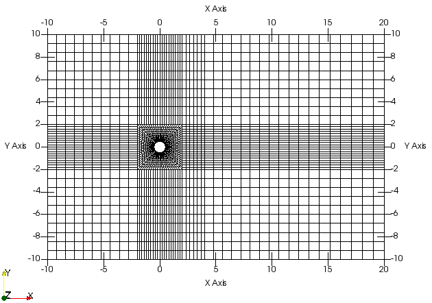
We aim to simulate the flow past a cylinder by solving the Compressible Navier Stokes equations. For our study we use the following free-stream parameters: A Mach number equal to M_∞ = 0.2, a Reynolds number Re_L=1 = 200 and Pr = 0.72, with the pressure set to p_∞ = 101325 Pa and the density equal to ρ = 1.225 Kg∕m³.

The flow domain is a rectangle of sizes [-10 20] x [-10 10]. The mesh consists of 639 quadrilaterals in which we applied the following boundary conditions (BCs): Non - slip isothermal wall on the cylinder surface, far - field at the bottom and top boundaries, inflow at the left boundary and outflow at the right boundary.

For the Navier-Stokes equations a non - slip condition must me applied to the velocity field at a solid wall, which corresponds to the cylinder for this problem. The cylinder wall is defined as an isothermal wall with imposed temperature T_wall = 300.15 K.

Inflow, Outflow and Farfield BCs:

In the Compressible Flow Solver the boundary conditions are weakly implemented- (i.e the BCs are applied to the fluxes). In the Euler equations, for farfield BCs, the flux is computed via a Riemann solver. The use of a Riemann solver for applying BCs implies the usage of a ghost point where it is necessary to apply a consistent ghost state, which is not always trivial. In evaluating the boundary, the Riemann solver takes automatically into account the eigenvalues (characteristic lines) of the Euler equations and therefore the problem is always well posed. This approach is equivalent to a characteristic approach where the corresponding Riemann invariants are computed and applied as BCs, taking into account if the boundary is an inflow or outflow. The method is also known as no-reflective BCs as it damps the spurious reflections from the boundaries.

The characteristic approach presented for the Euler equations for farfield boundaries, works also for the advective flux of the Navier-Stokes equations in regions where viscosity effects can be neglected. However, in our outflow case shedding is present, so viscosity effects become important. In this case, the characteristic treatment of the BCs generates spurious oscillations polluting the overall solution and leading to numerical instabilities. In order to avoid this, Nektar + + implements a method based on the so-called sponge terms, modifying the RHS of the compressible NS equations as follows:

(1.8)

Where σ(x) is a damping coefficient defined in a region x in proximity to the boundaries and u_ref is a known reference solution. The length and the shape of the damping coefficient depend on the problem being solved.

For further understanding of the boundary conditions implementation, please visit A Guide to the Implementation of Boundary Conditions in Compact High-Order Methods for Compressible Aerodynamics.

The initial condition is chosen to be that of a free flow field without the cylinder. If the solution greatly differs from the initial condition waves develop giving stability problems.

We successively setup the parameters of the problem (section 2.3). We finally run the solver (section 3) and post-process the data in order to visualise the results (section 4).