![]()
Figure 3.1: u′-component of the eigenmode
We will now perform transient growth analysis with a Krylov subspace of kdim=4. The
parameters and properties needed for this are present in the file bfs_tg.xml in
$NEKTUTORIAL/stability. In this case the Arpack library was used to compute the largest
eigenvalue of the system and the corresponding eigenmode. We will compute the maximum
growth for a time horizon of τ = 1, usually denoted G(1).
bfs_tg.xml session for performing transient growth analysis:
Set the EvolutionOperator to TransientGrowth.
Define a parameter FinalTime that is equal to 1 (this is the time horizon τ).
Set the number of steps (NumSteps) to be the ratio between the final time and the
time step.
Since the simulations take several iterations to converge, use the restart file
bfs_tg.rst for the initial condition. This file contains an eigenmode of the system.
Now run the simulation
IncNavierStokesSolver bfs_tg.xml
The terminal screen should look like this:
=======================================================================
                EquationType: UnsteadyNavierStokes
                Session Name: bfs_tg
                Spatial Dim.: 2
          Max SEM Exp. Order: 7
              Expansion Dim.: 2
             Projection Type: Continuous Galerkin
                   Advection: explicit
                   Diffusion: explicit
                   Time Step: 0.002
                No. of Steps: 500
         Checkpoints (steps): 500
            Integration Type: IMEXOrder2
=======================================================================
        Arnoldi solver type    : Arpack
        Arpack problem type    : LM
        Single Fourier mode    : false
        Beta set to Zero       : false
        Evolution operator     : TransientGrowth
        Krylov-space dimension : 4
        Number of vectors      : 1
        Max iterations         : 500
        Eigenvalue tolerance   : 1e-06
======================================================
Initial Conditions:
Field p not found.
Field p not found.
  - Field u: from file bfs_tg.rst
  - Field v: from file bfs_tg.rst
  - Field p: from file bfs_tg.rst
Writing: "bfs_tg_0.chk"
        Inital vector       : input file
Iteration 0, output: 0, ido=1 Steps: 500      Time: 1     CPU Time: 10.4384s
Writing: "bfs_tg_1.chk"
Time-integration  : 10.4384s
Steps: 500      Time: 29           CPU Time: 8.96463s
Writing: "bfs_tg_1.chk"
Time-integration  : 8.96463s
Writing: "bfs_tg.fld"
Iteration 1, output: 0, ido=1 Steps: 500      Time: 2     CPU Time: 8.90168s
Writing: "bfs_tg_1.chk"
Time-integration  : 8.90168s
Steps: 500      Time: 30           CPU Time: 8.90607s
Writing: "bfs_tg_1.chk"
Time-integration  : 8.90607s
Iteration 2, output: 0, ido=1 Steps: 500      Time: 3     CPU Time: 8.96875s
Writing: "bfs_tg_1.chk"
Time-integration  : 8.96875s
Steps: 500      Time: 31           CPU Time: 8.92276s
Writing: "bfs_tg_1.chk"
Time-integration  : 8.92276s
Iteration 3, output: 0, ido=1 Steps: 500      Time: 4     CPU Time: 8.92597s
Writing: "bfs_tg_1.chk"
Time-integration  : 8.92597s
Steps: 500      Time: 32           CPU Time: 8.96103s
Writing: "bfs_tg_1.chk"
Time-integration  : 8.96103s
Iteration 4, output: 0, ido=99
Converged in 4 iterations
Converged Eigenvalues: 1
         Magnitude   Angle       Growth      Frequency
EV: 0 3.23586     0           1.1743      0
Writing: "bfs_tg_eig_0.fld"
L 2 error (variable u) : 0.0118694
L inf error (variable u) : 0.0118647
L 2 error (variable v) : 0.0174185
L inf error (variable v) : 0.0244285
L 2 error (variable p) : 0.0109063
L inf error (variable p) : 0.0138423
Initially, the solution will be evolved forward in time using the operator A , then backward in time through the adjoint operator A*.
We can visualise graphically the optimal growth, recalling that the energy of the perturbation field at any given time t is defined by means of the inner product:
| (3.1) |
The solver can output the evolution of the energy of the perturbation in time by using the
ModalEnergy filter (defined in the FILTERS section of the XML file):
1<FILTER TYPE="ModalEnergy">
2   <PARAM NAME="OutputFile">energy</PARAM>
3   <PARAM NAME="OutputFrequency">10</PARAM>
4</FILTER>
This will write the energy of the perturbation every 10 time steps to the file energy.mld.
Repeating these simulations for different τ with the optimal initial perturbation as the initial
condition, it is possible to create a plot similar to figure 3.3. Each curve necessarily meets the
optimal growth envelope (denoted by the circles) at its corresponding value of τ, and never
exceeds it.
The $NEKTUTORIAL/energy folder contains the files bfs_energy_tau01.xml and
bfs_energy_tau20.xml, as well as the pre-computed optimal initial condition for
τ = 20 (bfs_energy_tau20.rst), with corresponding optimal growth of 2172.9.
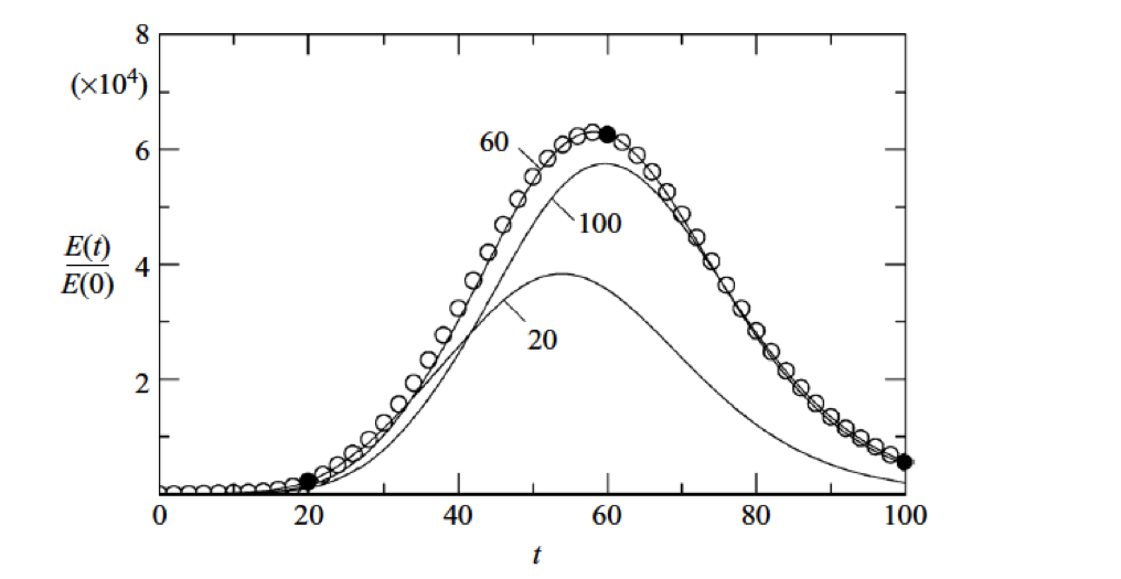
Use your favourite plotting program (e.g. MATLAB or GNUPlot) to read in the files produced by the energy filter and plot the normalised energy growth curves.
Standard driver. You should also use the Direct
evolution operator for this task, similar to the channel example.Examine your plot. Verify the energy at time t = τ matches the optimal growth in each case. Now examine the plot at time t = 1. Note that although the overall energy growth for the τ = 20 curve is far greater than the corresponding τ = 1 curve, the τ = 1 curve has greater growth at t = τ = 1.
