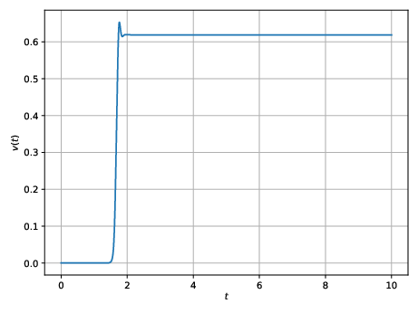
Figure 2.1 Time history of v(t) velocity component measured at (x,y) = (1.0,0.5).
This chapter will consider two-dimensional Rayleigh–Bénard convection in a box of aspect ratio 2.02. At the top and bottom walls, we employ a no-slip boundary condition for the velocity field and a conducting boundary condition for the temperature field. At the sidewalls, we set periodic boundary conditions for both fields. We will compare our results with Clever and Busse (J. Fluid Mech., 1974; 65:625-645) for Ra = 5000, Pr = 0.71, and Lx = 2π∕3.117 = 2.02.
In the folder $NEKTUTORIAL/DNS/Ra_5e3_Pr_0p71 you will find the file rbc-DNS.xml which
contains the geometry along with the necessary parameters to solve the problem. The
GEOMETRY section is responsible for defining the mesh of the problem, and it is automatically
generated, as demonstrated in the preceding task. Within the EXPANSIONS section, the
expansion type and order are specified. An expansion basis is applied to a geometric
composite, where composite refers to a collection of mesh entities. The $NEK/NekMesh utility
always includes a default entry, and in this case, the composite C[0] represents the set of all
elements. The FIELDS attribute indicates the fields for which this expansion is applicable, and
the TYPE attribute designates the type of polynomial basis functions used in the expansion.
For example,
1<EXPANSIONS>
2   <E COMPOSITE="C[0]" NUMMODES="10" FIELDS="u,v,T,p"
3   TYPE="GLL_LAGRANGE_SEM" />
4</EXPANSIONS>.
To finalise the problem definition and facilitate solution generation, we define a section named
CONDITIONS within the session file. Specifically, the CONDITIONS section encompasses the
following entries:
Solver information (SOLVERINFO) such as the equation, the projection type, the
evolution operator, and the analysis driver to use, along with other properties.
The solver properties are specified as quoted attributes and have the form
1<SOLVERINFO>
2   <I PROPERTY="[STRING]" VALUE="[STRING]" />
3   ...
4</SOLVERINFO>
SOLVERINFO section of rbc-DNS.xml:
Note: The bits to be completed are identified by …in this file.
The parameters (PARAMETERS) are specified as name-value pairs:
1<PARAMETERS>
2   <P> [KEY] = [VALUE] </P>
3   ...
4</PARAMETERS>
Ra, that represents the Rayleigh number, and
Pr, which represents the Prandtl number. Now set the Rayleigh number to 5000 and the
Prandtl number to 0.71 - i.e.<P> Ra = 5000 </P><P> Pr = 0.71 </P>The declaration of the variable(s) (VARIABLES).
1<VARIABLES>
2        <V ID="0"> u </V>
3        <V ID="1"> v </V>
4        <V ID="2"> T </V>
5        <V ID="3"> p </V>
6</VARIABLES>
Defining boundary regions (BOUNDARYREGIONS) involves specifying composites from
the GEOMETRY section and the associated conditions applied to these boundaries
(BOUNDARYCONDITIONS). The format for boundary conditions imposed on a region
must be in accordance with the conditions outlined for each variable in the VARIABLES
section to establish a well-posed problem. The REF attribute associated with a boundary
condition region ought to align with the ID="[INDEX]" of the intended boundary
region outlined in the BOUNDARYREGIONS section. For example, to model a
hot bottom plate corresponding to REF="0", we set the following condition:
1<REGION REF="0">
2   <D VAR="u" VALUE="0" />
3   <D VAR="v" VALUE="0" />
4   <D VAR="T" VALUE="1" />
5   <N VAR="p" USERDEFINEDTYPE="H" VALUE="0" />
6</REGION>
REF="1" in the session
file.The specification of (time- and) space-dependent functions (FUNCTION), involves defining
functions in terms of x, y, z, and t, encompassing aspects like initial conditions and
forcing functions. The VARIABLES denote the components of the particular function in a
specified direction.
1<FUNCTION NAME="[NAME]">
2   <E VAR="[VARIABLE_1]" VALUE="[EXPRESSION]"/>
3   <E VAR="[VARIABLE_2]" VALUE="[EXPRESSION]"/>
4   ...
5</FUNCTION>
Next, we apply the buoyancy force in the vertical direction, with gravity acting downward. This is implemented by defining the following function as the body force.
1<FUNCTION NAME="BodyForce">
2      <E VAR="u" VALUE="0" EVARS="uvT">
3      <E VAR="v" VALUE="Ra*Pr*T" EVARS="uvT" />
4      <E VAR="T" VALUE="0" EVARS="uvT" />
5</FUNCTION>
Note that for using the body force you need the following additional tag outside the section
CONDITIONS:
1<FORCING>
2   <FORCE TYPE="Body">
3      <BODYFORCE> BodyForce </BODYFORCE>
4   </FORCE>
5</FORCING>
We also wish to monitor the simulation progress. To achieve this, we plan to record flow
quantities at the location (x,y) = (1.0,0.5). For this purpose, we incorporate a filter called
HistoryPoints in the session file as follows:
1   <FILTERS>
2      <FILTER TYPE="HistoryPoints">
3        <PARAM NAME="OutputFile">rbc</PARAM>
4        <PARAM NAME="OutputFrequency">10</PARAM>
5        <PARAM NAME="Points">
6           1.0 0.5 0
7        </PARAM>
8      </FILTER>
9   </FILTERS>
This completes the specification of the problem.
$NEK/IncNavierStokesSolver rbc-DNS.xml
Next, we want to visualise the steady solution. Specifically, we need to convert the .fld file
into a format readable by a visualisation post-processing tool. In this tutorial we decided to
convert the .fld file into a VTK format and to use the open-source visualisation package
called Visit.
$NEK/FieldConvert rbc-DNS.xml rbc-DNS.fld rbc-DNS.vtu
Now open Visit and use File ->Open, to select the VTK file. Next, you can plot different fields.
To validate our results, we will calculate the Nusselt number (Nu), representing the ratio of the total heat flux (convective plus conductive) to the conductive heat flux at the plate. The Nusselt number is expressed as follows1 :
Nu = - ∫ ∫
 dx. dx. | (2.5) |
For the calculation of the Nusselt number, we will use the FieldCovert and NekMesh utility.
We will follow the following steps:
Extract the wall boundary surface in a xml file using the NekMesh utility as:
NekMesh -m extract:surf=1 rbc-DNS.xml rbc_surf.xml
NUMODES and the polynomial basis functions according to
the session file in rbc-DNS.xml.Compute  , and remove all unnecessary fields.
FieldConvert -m gradient rbc-DNS.xml rbc-DNS.fld temp_1.fld
FieldConvert -m removefield:fieldname="u,v,T,p,u_x,u_y,\\
v_x,v_y,T_x,p_x,p_y" rbc-DNS.xml temp_1.fld dT_dy.fld
Next, extract  at the top boundary.
FieldConvert -m extract:bnd=0 rbc-DNS.xml dT_dy.fld dT_dy_bnd.fld
Finally, we will compute  ∫
∫
 dx using
 mean utility.
FieldConvert -m mean rbc_surf.xml dT_dy_bnd_b0.fld stdout
Above command gives the following output:
Domain length : 2.02
Integral (variable T_y) : -4.26191
Mean (variable T_y) : -2.10986
Now since

Our calculation of the Nusselt number match very well with that of Clever and Busse (J. Fluid Mech., 1974; 65:625-645), which is 2.112.
rbc-DNS.xml change the
values of Ra and Pr, and again run the solver to compute the Nusselt number (your results
should match with Table (2.1).
This completes the tutorial.