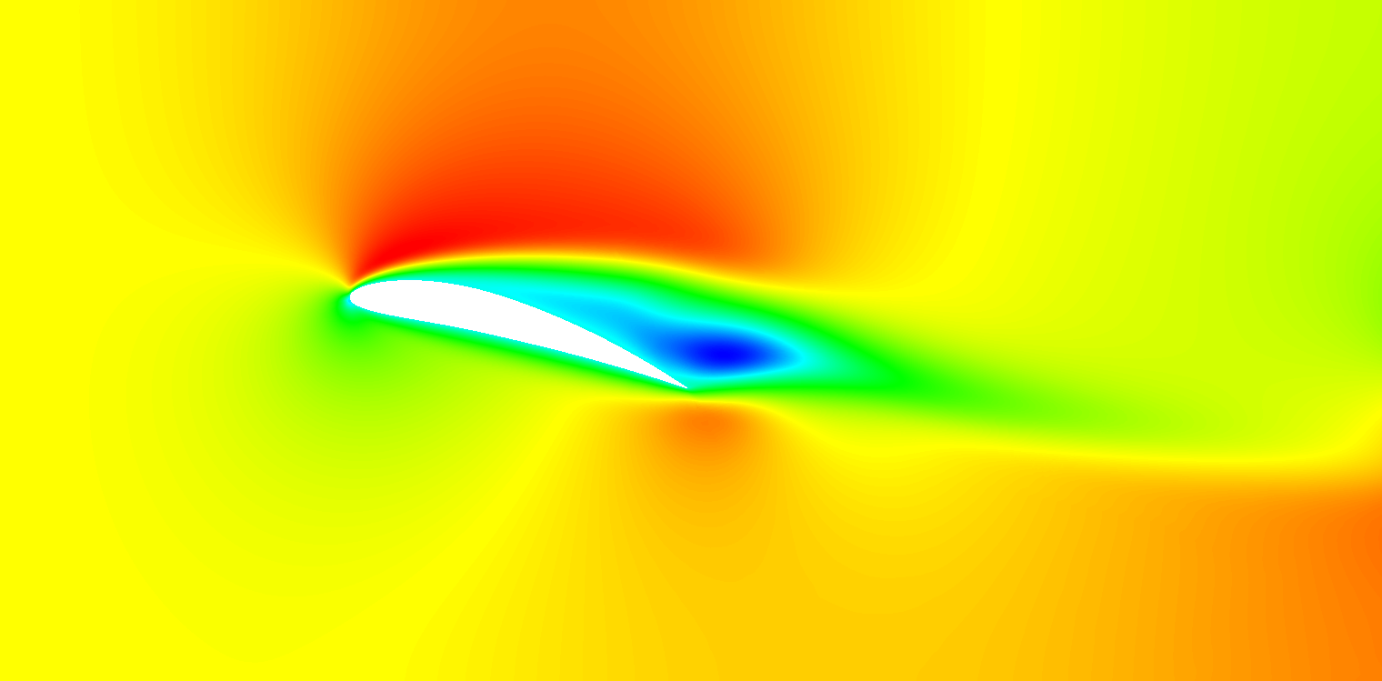
Figure 2.1: Visualisation of streamwise velocity field at t = 2.5.
An additional feature of the 2D capabilities of NekMesh is to generate meshes of NACA wings
without the need for a CAD file. By listing the CADFile parameter as a 4 digit NACA code in
the .mcf, NekMesh will generate the NACA wing. Additional parameters about the domain
are required, that define the minimum and maximum x- and y-coordinates for the grid and the
angle of attack of the wing:
1   <P PARAM="Xmin" VALUE="-1.0" />
2   <P PARAM="Ymin" VALUE="-1.0" />
3   <P PARAM="Xmax" VALUE="3.0" />
4   <P PARAM="Ymax" VALUE="1.0" />
5   <P PARAM="AOA" VALUE="15.0" />
The mesh we make is for a simple NACA 6412 profile in a rectangular domain.
$NEK/NekMesh naca.mcf naca.xml
More details about the generation process can be seen by enabling the verbose command line
option -v:
$NEK/NekMesh -v naca.mcf naca.xml
This will produce a Nektar++ mesh, which we now need to visualise.
$NEK/FieldConvert naca.xml naca.dat
or, for VTK output, for visualisation in ParaView or VisIt, run the command
$NEK/FieldConvert naca.xml naca.vtu
As these meshes are converted to a linear mesh, since this is what the visualisation software
supports, the curved elements can look quite faceted. To counteract this, we can add an
optional -nX command line option to FieldConvert, which increases the number of
subdivisions used to view the elements through interpolation.
$NEK/FieldConvert -n 8 naca.xml naca.vtu
and visualise the output, which should now look far smoother around the aerofoil’s leading edge and give a better visualisation of the high-order elements.
The .mcf has already been configured for the generation of a sufficiently fine mesh. Among
others, it includes a boundary layer mesh as well as a refinement region in the wake
of the aerofoil. We can now try to run some simulations on this mesh. A session
file session_naca.xml for the aerofoil mesh is provided, which will execute a low
Reynolds number incompressible simulation. The resulting flow field should look like in
Fig. 2.1.
$NEK/IncNavierStokesSolver naca.xml session_naca.xml
Process the final flow field visualisation with
$NEK/FieldConvert naca.xml naca.fld naca.vtu
and visualise the results.
It is possible to visualise the unsteady flow by getting the solver to write checkpoint files every
certain number of timesteps using the Checkpoint filter. The output frequency is controlled
by the OutputFrequency parameter.
1<FILTERS>
2   <FILTER TYPE="Checkpoint">
3      <PARAM NAME="OutputFrequency">50</PARAM>
4   </FILTER>
5</FILTERS>
$NEK/IncNavierStokesSolver naca.xml session_naca.xml
Finally, process these checkpoint files for visualisation by using the command
for i in {0..100}; do $NEK/FieldConvert naca.xml naca_${i}.chk naca_${i}.vtu;
 done
Note that this is a bash command – if you use an alternative shell, such as tcsh, you may
need to alter this syntax. Load the files into your visualiser as a group, and use the frame
functions to view the flow as an unsteady animation.
Following these first 2 tutorials on two-dimensional high-order mesh generation using NekMesh, the reader should now be able to modify the mesh configuration file according to their needs.