The CompressibleFlowSolver allows us to solve the unsteady compressible Euler and Navier-Stokes equations for 1D/2D/3D problems using a discontinuous representation of the variables. In the following we describe both the compressible Euler and the Navier-Stokes equations.
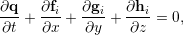
The Euler equations can be expressed as a hyperbolic conservation law in the form
|
| (7.1) |
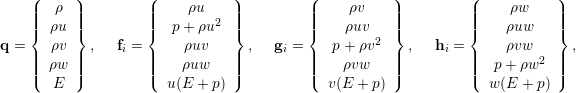
where q is the vector of the conserved variables, fi = fi(q), gi = gi(q) and hi = hi(q) are the vectors of the inviscid fluxes
 | (7.2) |
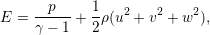
where ρ is the density, u, v and w are the velocity components in x, y and z directions, p is the pressure and E is the total energy. In this work we considered a perfect gas law for which the pressure is related to the total energy by the following expression
 | (7.3) |
where γ is the ratio of specific heats.
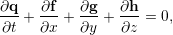
The Navier-Stokes equations include the effects of fluid viscosity and heat conduction and are consequently composed by an inviscid and a viscous flux. They depend not only on the conserved variables but also, indirectly, on their gradient. The second order partial differential equations for the three-dimensional case can be written as:
 | (7.4) |
where q is the vector of the conserved variables, f = f(q,∇(q)), g = g(q,∇(q)) and h = h(q,∇(q)) are the vectors of the fluxes which can also be written as:
 | (7.5) |
where fi, gi and hi are the inviscid fluxes of Eq. (7.2) and fv, gv and hv are the viscous fluxes which take the following form:
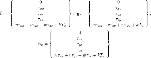 | (7.6) |
where τxx, τxy, τxz, τyx, τyx, τyy, τyz, τzx, τzy and τzz are the components of the stress tensor1
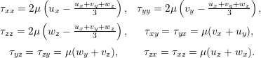 | (7.7) |
where μ is the dynamic viscosity calculated using the Sutherland’s law and k is the thermal conductivity.
In Nektar++ the spatial discretisation of the Euler and of the Navier-Stokes equations is projected in the polynomial space via a discontinuous projection. Specifically we make use either of the discontinuous Galerkin (DG) method or the Flux Reconstruction (FR) approach. In both the approaches the physical domain Ω is divided into a mesh of N non-overlapping elements Ωe and the solution is allowed to be discontinuous at the boundary between two adjacent elements. Since the Euler as well as the Navier-Stokes equations are defined locally (on each element of the computational domain), it is necessary to define a term to couple the elements of the spatial discretisation in order to allow information to propagate across the domain. This term, called numerical interface flux, naturally arises from the discontinuous Galerkin formulation as well as from the Flux Reconstruction approach.
For the advection term it is common to solve a Riemann problem at each interface of the computational domain through exact or approximated Riemann solvers. In Nektar++ there are different Riemann solvers, one exact and nine approximated. The exact Riemann solver applies an iterative procedure to satisfy conservation of mass, momentum and energy and the equation of state. The left and right states are connected either with the unknown variables through the Rankine-Hugoniot relations, in the case of shock, or the isentropic characteristic equations, in the case of rarefaction waves. Across the contact surface, conditions of continuity of pressure and velocity are employed. Using these equations the system can be reduced to a non-linear algebraic equation in one unknown (the velocity in the intermediate state) that is solved iteratively using a Newton method. Since the exact Riemann solver gives a solution with an order of accuracy that is related to the residual in the Newton method, the accuracy of the method may come at high computational cost. The approximated Riemann solvers are simplifications of the exact solver.
Concerning the diffusion term, the coupling between the elements is achieved by using a local discontinuous Galerkin (LDG) approach as well as five different FR diffusion terms.
The boundary conditions are also implemented by exploiting the numerical interface fluxes just mentioned. For a more detailed description of the above the interested reader can refer to [6] and [14].