Example files for the ADRSolver are provided in solvers/ADRSolver/Examples
In this example, it will be demonstrated how the Advection equation can be solved on a one-dimensional domain.
We consider the hyperbolic partial differential equation:
|
| (6.2) |
where f = au is the advection flux.
The input for this example is given in the example file Advection1D.xml
The geometry section defines a 1D domain consisting of 10 segments. On each segment an expansion consisting of 4 Lagrange polynomials on the Gauss-Lobotto-Legendre points is used as specified by
Since we are solving the unsteady advection problem, we must specify this in the solver information. We also choose to use a discontinuous flux-reconstruction projection and use a Runge-Kutta order 4 time-integration scheme.
We choose to advect our solution for 20 time units with a time-step of 0.01 and so provide the following parameters
We also specify the advection velocity. We first define dummy parameters
and then define the actual advection function as
Two boundary regions are defined, one at each end of the domain, and periodicity is enforced
Finally, we specify the initial value of the solution on the domain
To visualise the output, we can convert it into either TecPlot or VTK formats
In this example, it will be demonstrated how the Helmholtz equation can be solved on a two-dimensional domain.
We consider the elliptic partial differential equation:
 | (6.3) |
where ∇2 is the Laplacian and λ is a real positive constant.
The input for this example is given in the example file Helmholtz2D_modal.xml
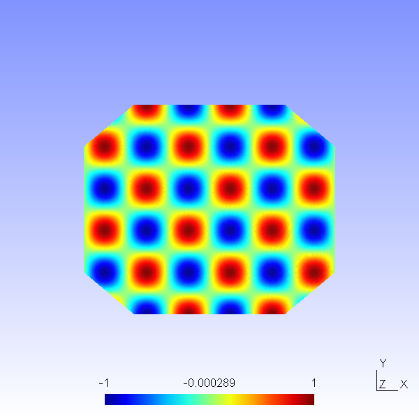
The geometry for this problem is a two-dimensional octagonal plane containing both triangles and quadrilaterals. Note that a mesh composite may only contain one type of element. Therefore, we define two composites for the domain, while the rest are used for enforcing boundary conditions.
For both the triangular and quadrilateral elements, we use the modified Legendre basis with 7 modes (maximum polynomial order is 6).
Only one parameter is needed for this problem. In this example λ = 1 and the Continuous Galerkin Method is used as projection scheme to solve the Helmholtz equation, so we need to specify the following parameters and solver information.
All three basic boundary condition types have been used in this example: Dirichlet, Neumann and Robin boundary. The boundary regions are defined, each of which corresponds to one of the edge composites defined earlier. Each boundary region is then assigned an appropriate boundary condition.
We know that for f = −(λ + 2π2)sin(πx)cos(πy), the exact solution of the two-dimensional Helmholtz equation is u = sin(πx)cos(πy). These functions are defined specified to initialise the problem and verify the correct solution is obtained by evaluating the L2 and Linf errors.
This execution should print out a summary of input file, the L2 and Linf errors and the time spent on the calculation.
Simulation results are written in the file Helmholtz2D_modal.fld. We can choose to visualise the output in Gmsh
which generates the file Helmholtz2D_modal.vtu which can be visualised and is shown in Fig. 6.1
The following example demonstrates the application of the ADRsolver for modelling advection dominated mass transport in a straight pipe. Such a transport regime is encountered frequently when modelling mass transport in arteries. This is because the diffusion coefficient of small blood borne molecules, for example oxygen or adenosine triphosphate, is very small O(10−10).
The governing equation for modelling mass transport is the unsteady advection diffusion equation:
 + v∇u + ϵ∇2u = 0 + v∇u + ϵ∇2u = 0 |
For small diffusion coefficient, ϵ, the transport is dominated by advection and this leads to a very fine boundary layer adjacent to the surface which must be captured in order to get a realistic representation of the wall mass transfer processes. This creates problems not only from a meshing perspective, but also numerically where classical oscillations are observed in the solution due to under-resolution of the boundary layer.
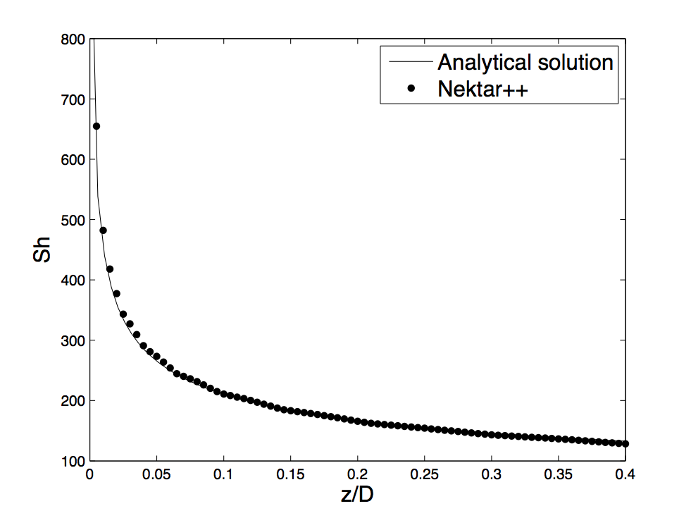
The Graetz-Nusselt solution is an analytical solution of a developing mass (or heat) transfer boundary layer in a pipe. Previously this solution has been used as a benchmark for the accuracy of numerical methods to capture the fine boundary layer which develops for high Peclet number transport (the ratio of advection to diffusion). The solution is derived based on the assumption that the velocity field within the mass transfer boundary layer is linear i.e. the Schmidt number (the relative thickness of the momentum to mass transfer boundary layer) is sufficiently large. The analytical solution for the non-dimensional mass transfer at the wall is given by:
Sh(z) = 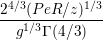 , , |
Pe =  |
In the following we will numerically solver mass transport in a pipe and compare the calculated mass transfer at the wall with the Graetz-Nusselt solution. The Peclet number of the transport regime under consideration is 750000, which is physiologically relevant.
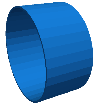
The geometry under consideration is a pipe of radius, R = 0.5 and length l = 0.5
Since the mass transport boundary layer will be confined to a very small layer adjacent to the wall we do not need to mesh the interior region, hence the mesh consists of a layer of ten prismatic elements over a thickness of 0.036R. The elements progressively grow over the thickness of domain.
In this example we utilise heterogeneous polynomial order, in which the polynomial order normal to the wall is higher so that we avoid unphysical oscillations, and hence the incorrect solution, in the mass transport boundary layer. To do this we specify explicitly the expansion type, points type and distribution in each direction as follows:
The above represents a quadratic polynomial order in the azimuthal and streamwise direction and 4th order polynomial normal to the wall for a prismatic element.
We choose to use a continuous projection and an first-order implicit-explicit time-integration
scheme. The DiffusionAdvancement and AdvectionAdvancement parameters specify how
these terms are treated.
We integrate for a total of 30 time units with a time-step of 0.0005, necessary to keep the simulation numerically stable.
The value of the ϵ parameter is ϵ = 1∕Pe
The analytical solution represents a developing mass transfer boundary layer in a pipe. In order to reproduce this numerically we assume that the inlet concentration is a uniform value and the outer wall concentration is zero; this will lead to the development of the mass transport boundary layer along the length of the pipe. Since we do not model explicitly the mass transfer in the interior region of the pipe we assume that the inner wall surface concentration is the same as the inlet concentration; this assumption is valid based on the large Peclet number meaning the concentration boundary layer is confined to the region in the immediate vicinity of the wall. The boundary conditions are specified as follows in the input file:
The velocity field within the domain is fully devqeloped pipe flow (Poiseuille flow), hence we can define this through an analytical function as follows:
We assume that the initial domain concentration is uniform everywhere and the same as the inlet. This is defined by,
To compare with the analytical expression we numerically calculate the concentration gradient at the surface of the pipe. This is then plotted against the analytical solution by extracting the solution along a line in the streamwise direction, as shown in Fig. 6.3.