 | (10.1a) |
 | (10.1b) |
A useful tool implemented in Nektar++ is the incompressible Navier Stokes solver that allows to solve the governing equation for viscid Newtonians fluid using two different algorithms.
where V is the velocity, p the pressure and ν the kinematic viscosity. The first approach uses a
splitting/projection method where the velocity matrix system and the pressure are typically
decoupled. Splitting schemes are typically favourite for their numerical efficiency since for
a Newtonian fluid the velocity and pressure are handled independently, requiring
the solution of three (in two dimensions) elliptic systems of rank N (opposed to a
single system of rank 3N solved in the Stokes problem). However, a drawback of this
approach is the splitting scheme error which is introduced when decoupling the
pressure and the velocity system, although this can be made consistent with the
overall temporal accuracy of the scheme by appropriate discretisation of the pressure
boundary conditions. When the incompressible Navier-Stokes equations are solved
using the velocity correction splitting scheme, a stiffly-stable time integration is
applied (derived from the work of Karniadakis, Israeli and Orszag [16], see also
Guermond and Shen [13]). Briefly, the time integration scheme consists of the following
steps:
![∑J −1 αq
V˜-−---q=0-γ0-Vn−-q J∑−1βq- n−q n+1
Δt = γ0[− (V ⋅∇ )V ] + f
q=0](user-guide70x.png) | (10.2) |
 | (10.3) |
with consistent Neumann boundary conditions prescribed as
![n+1 [ n+1 J− 1 J− 1 ]
-∂p = − ∂V-- + ν∑ βq(∇ × ∇ × V )n−q + ∑ βq[(V ⋅∇)V ]n−q ⋅n
∂n ∂t q=0 q=0](user-guide72x.png) | (10.4) |
and on the outflow boundary, either setting pn+1 = 0 or using high order Dirichlet boundary condition, which is given as[9]
 | (10.5) |
with a step function defined by So(n ⋅V) =  (1 − tanh
  ), where V0 is
the characteristic velocity scale and δ is a non-dimensional positive constant
chosen to be sufficiently small. fb is the forcing term in this case the analytical
conditions can be given but if these are not known explicitly, it is set to zero, i.e.
fb = 0.
), where V0 is
the characteristic velocity scale and δ is a non-dimensional positive constant
chosen to be sufficiently small. fb is the forcing term in this case the analytical
conditions can be given but if these are not known explicitly, it is set to zero, i.e.
fb = 0.
 | (10.6) |
 | (10.7) |
with the outflow boundary conditions either set as n ⋅∇Vn+1 = 0 or as high order Neumann boundary conditions prescribed by[9]:
![1[ 1 J−∑ 1 J∑−1 J∑−1 ]
n ⋅∇Vn+1 = --pn+1n + --| Vn −q |2 So (n ⋅ Vn− q)n − ν (∇ ⋅Vn −q)n+ fnb+1
ν 2 q=0 q=0 q=0](user-guide78x.png) | (10.8) |
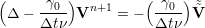
Here, J is the integration order and γ0, αq, βq are the stiffly stable time integration coefficients given in the table below.
 | (10.9) |
This multi-step implicit-explicit splitting scheme decouples the velocity field V from the pressure p, leading to an explicit treatment of the advection term and an implicit treatment of the pressure and the diffusion term.
It is possible to use difference time steps in the velocity correction scheme using a substepping [28] or auxiliary semi-Lagrangian approach [35]. Originally the scheme was proposed by Maday, Patera and Ronquist who referred to as an operator-integration-factor splitting method [20]
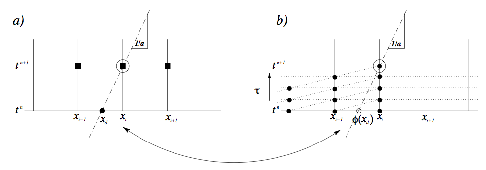
A schematic of the approach can be understood from figure 10.1.2 where we observe that
smaller time steps can be used for the explicit advection steps whilst a larger overall time step
is adopted for the more expensive implicit solve for the diffusion operator. More details of the
implementation can be found in [35] and [28]. In the following sections we outline the
parameters that can be used to set up this scheme. Since the explicit part is advanced using a
DG scheme it is necessary to use a Mixed_CG_Discontinuous expansion with this
option.
$NEKHOME/Solver/IncNavierStokesSolver/Tests/ directory. For exmaple
the test cases KovaFlow_SubStep_2order.xml, Hex_Kovasnay_SubStep.xml and
Tet_Kovasnay_SubStep.xml
The second approach consists of directly solving the matrix problem arising from the discretization of the Stokes problem. The direct solution of the Stokes system introduces the problem of appropriate spaces for the velocity and the pressure systems to satisfy the inf-sup condition and it requires the solution of the full velocity-pressure system. However, if a discontinuous pressure space is used then all but the constant mode of the pressure system can be decoupled from the velocity. When implementing this approach with a spectral/hp element discretization, the remaining velocity system may then also be statically condensed to decouple the so called interior elemental degrees of freedom, reducing the Stokes problem to a smaller system expressed on the elemental boundaries. The direct solution of the Stokes problem provides a very natural setting for the solution of the pressure system which is not easily dealt with in a splitting scheme. Further, the solution of the full coupled velocity system allows the introduction of a spatially varying viscosity, which arise for non-Newtonian flows, with only minor modifications.
We consider the weak form of the Stokes problem for the velocity field boldsymbolu = [u,v]T and the pressure field p:
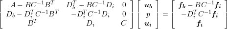
where the components of A,B and C are ∇ϕb,ν∇ub, ∇ϕb,ν∇ui and ∇ϕi,ν∇ui and the components Db and Di are q,∇ub and q,∇ui. The indices b and i refer to the degrees of freedom on the elemental boundary and interior respectively. In constructing the system we have lumped the contributions form each component of the velocity field into matrices A,B and C. However, we note that for a Newtonian fluid the contribution from each field is decoupled. Since the interior degrees of freedom of the velocity field do not overlap, the matrix C is block diagonal and to take advantage of this structure we can statically condense out the C matrix to obtain the system:
 | (10.11) |
To extend the above Stokes solver to an unsteady Navier-Stokes solver we first introduce the unsteady term, ∂u∕∂t, into the Stokes problem. This has the principal effect of modifying the weak Laplacian operator ∇ϕ,ν∇u] into a weak Helmholtz operator ∇ϕ,ν∇u) −λ(ϕ,u where λ depends on the time integration scheme. The second modification requires the explicit discretisation of the non-linear terms in a similar manner to the splitting scheme and this term is then introduced as the forcing term f. For more details see [1, 29].
Hydrodynamic stability is an important part of fluid-mechanics that has a relevant role in understanding how an unstable flow can evolve into a turbulent state of motion with chaotic three-dimensional vorticity fields and a broad spectrum of small temporal and spatial scales. The essential problems of hydrodynamic stability were recognised and formulated in 19th century, notably by Helmholtz, Kelvin, Rayleigh and Reynolds.
Conventional linear stability assumes a normal representation of the perturbation fields that can be represented as independent wave packets, meaning that the system is self-adjoint. The main aim of the global stability analysis is to evaluate the amplitude of the eigenmodes as time grows and tends to infinity. However, in most industrial applications, it is also interesting to study the behaviour at intermediate states that might affects significantly the functionality and performance of a device. The study of the transient evolution of the perturbations is seen to be strictly related to the non-normality of the linearised Navier-Stokes equations, therefore the normality assumptiong of the system is no longer assumed. The eigenmodes of a non-normal system do not evolve independently and their interaction is responsible for a non-negligible transient growth of the energy. Conventional stability analysis generally does not capture this behaviour, therefore other techniques should be used.
A popular approach to study the hydrodynamic stability of flows consists in performing a direct numerical simulation of the linearised Navier-Stokes equations using iterative methods for computing the solution of the associated eigenproblem. However, since linearly stable flows could show a transient increment of energy, it is necessary to extend this analysis considering the combined effect of the direct and adjoint evolution operators. This phenomenon has noteworthy importance in several engineering applications and it is known as transient growth.
In Nektar++ it is then possible to use the following tools to perform stability analysis:
The equations that describe the evolution of an infinitesimal disturbance in the flow can be derived decomposing the solution into a basic state (U,p) and a perturbed state U + εu′ with ε « 1 that both satisfy the Navier-Stokes equations. Substituting into the Navier Stokes equations and considering that the quadratic terms u′⋅∇u′can be neglected, we obtain the linearised Navier-Stokes equations:
The linearised Navier-Stokes equations are identical in form to the non-linear equation, except for the non-linear advection term. Therefore the numerical techniques used for solving Navier-Stokes equations can still be applied as long as the non-linear term is substituted with the linearised one. It is possible to define the linear operator that evolved the perturbation forward in time:
 | (10.13) |
Let us assume that the base flow U is steady, then the perturbations are autonomous and we can assume that:
 | (10.14) |
Then we obtain the associated eigenproblem:
 | (10.15) |
The dominant eigenvalue determines the behaviour of the flow. If it the real part is positive there exists exponentially growing solutions, conversely if every single eigenvalues has negative real part then the flow is linearly stable. If the real part of the eigenvalue is zero, it is present a bifurcation point.
The adjoint of a linear operator is one of the most important concept in functional analysis and has an it has important role to tackle the transition to turbulence. Let us write the linearised Navier-Stokes equation in a compact form:
 | (10.16) |
The adjoint operator (H∗ is defines as:
 | (10.17) |
Integrating by parts and employing the divergence theorem, it is possible to express the adjoint equations:
The adjoint fields are in fact related to the concept of receptivity. The value of the adjoint velocity at a point in the flow indicates the response that arises from an unsteady momentum source at that point. The adjoint pressure and the adjoint stream function play instead the same role for mass and vorticity sources respectively. Therefore, the adjoint modes can be seen as a powerful tool to understand where to act in order to ease/inhibit the transition.
Transient growth is a phenomenon that occurs when a flow that is linearly stable, but whose perturbations exhibit a non-negligible transient response due to regions of localised convective instabilities. This situation is common in many engineering applications, for example in open flows where the geometry is complex, producing a steep variation of the base flow. Therefore, the main question to answer is if it exists a bounded solution that exhibit large growth before inevitably decaying. Let us introduce a norm to quantify the size of a perturbation. It is physically meaningful to use the total kinetic energy of a perturbation on the domain Ω. This is convenient because it is directly associated with the standard-L2 inner product:
 | (10.19) |
where σ =  . This is no other that the singular value decomposition of A(τ). The
phenomenology of the transient growth can be explained considering the non-normality of the
linearised Navier-Stokes evolution operator. This can be simply understood using the simple
geometric example showed in figure 10.1.4.3. Let us assume a unit-length vector f
represented in a non-orthogonal basis .This vector is defined as the difference of the
nearly collinear vectors Φ1 and Φ2. With the time progression, the component of
these two vectors decrease respectively by 20% and 50%. The vector f increases
substantially in length before decaying to zero. Thus, the superposition of decaying
non-orthogonal eigenmode can produce in short term a growth in the norm of the
perturbations.
. This is no other that the singular value decomposition of A(τ). The
phenomenology of the transient growth can be explained considering the non-normality of the
linearised Navier-Stokes evolution operator. This can be simply understood using the simple
geometric example showed in figure 10.1.4.3. Let us assume a unit-length vector f
represented in a non-orthogonal basis .This vector is defined as the difference of the
nearly collinear vectors Φ1 and Φ2. With the time progression, the component of
these two vectors decrease respectively by 20% and 50%. The vector f increases
substantially in length before decaying to zero. Thus, the superposition of decaying
non-orthogonal eigenmode can produce in short term a growth in the norm of the
perturbations.
To compute linear stability analysis, the choice of the base flow, around which the system will be linearised, is crucial. If one wants to use the steady-state solution of the Navier-Stokes equations as base flow, a steady-state solver is implemented in Nektar++. The method used is the encapsulated formulation of the Selective Frequency Damping method [15]. Unstable steady base flows can be obtained with this method. The SFD method is based on the filtering and control of unstable temporal frequencies within the flow. The time continuous formulation of the SFD method is
 | (10.20) |
where q represents the problem unknown(s), the dot represents the time derivative, NS represents the Navier-Stokes equations, χ ∈ ℝ+ is the control coefficient, is a filtered version of q, and Δ ∈ ℝ+∗ is the filter width of a first-order low-pass time filter. The steady-state solution is reached when q = .
The convergence of the method towards a steady-state solution depends on the choice of the parameters χ and Δ. They have to be carefully chosen: if they are too small, the instabilities within the flow can not be damped; but if they are too large, the method may converge extremely slowly. If the dominant eigenvalue of the flow studied is known (and given as input), the algorithm implemented can automatically select parameters that ensure a fast convergence of the SFD method. Most of the time, the dominant eigenvalue is not know, that is why an adaptive algorithm that adapts χ and Δ all along the solver execution is also implemented.
Note that this method can not be applied for flows with a pure exponential growth of the instabilities (e.g. jet flow within a pipe). In other words, if the frequency of the dominant eigenvalue is zero, then the SFD method is not a suitable tool to obtain a steady-state solution.