12.4 Examples

12.4.1 Human Vascular Network

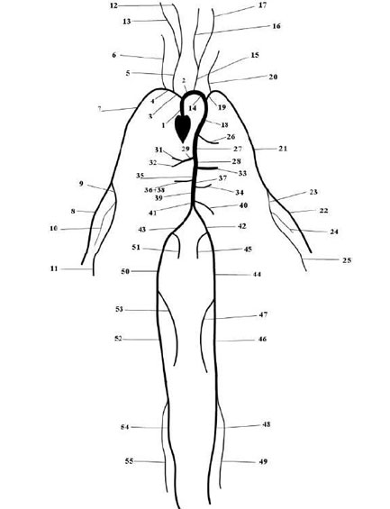
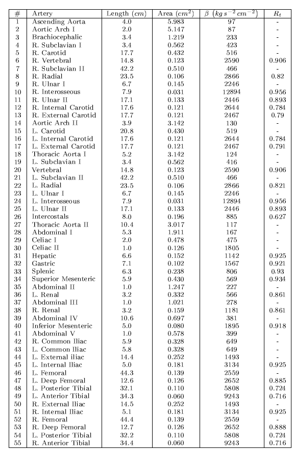
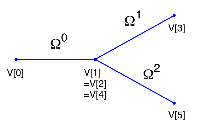
The Pulse Wave Solver is also capable of handling more complex networks, such as a complete human arterial tree proposed by Westerhof et al. [34]. In this example, we will use the refined data from [30] and set up the network shown in the figure in the right. We will explain how bifurcations are set correctly and how each arterial segment gets its correct physiological data.


PIC PIC


First, we will set up the mesh where each arterial segment is represented by one element and two vertices respectively. Then, we will subdivide the mesh into different subdomains by using the <COMPOSITE> section. Here, each arterial segment is described by the contained elements and its first and last vertex.

The mesh connectivity is specified during the creation of elements by indicating the starting vertex and ending vertex of each individual artery segment. Shared vertices are used to describe bifurcations, junctions and mergers between different artery segments in the network.

The composites are then used to specify the two adjoining segments of an artery, where the first segment merely allows for description of the connectivity.

1<GEOMETRY DIM="1" SPACE="1"> 
2    <VERTEX> 
3        <V ID="0"> 0.000e+00 0.000e+00 0.000e+00</V> <!-- 1 --> 
4        <V ID="1"> 4.000e+00 0.000e+00 0.000e+00</V> 
5 
6        <V ID="2"> 4.000e+00 0.000e+00 0.000e+00</V> <!-- 2 --> 
7        <V ID="3"> 6.000e+00 0.000e+00 0.000e+00</V> 
8 
9        <V ID="4"> 4.000e+00 0.000e+00 0.000e+00</V> <!-- 3 --> 
10        <V ID="5"> 7.400e+00 0.000e+00 0.000e+00</V> 
11           . 
12           . 
13           . 
14        <V ID="108"> 109.100e+00 -45.000e+00 0.000e+00</V> <!-- 55 --> 
15        <V ID="109"> 143.500e+00 -45.000e+00 0.000e+00</V> 
16    </VERTEX> 
17    <ELEMENT> 
18        <S ID="0">    0     1 </S> 
19        <S ID="1">    1     2 </S> 
20        <S ID="2">    1     4 </S> 
21        <S ID="3">    2     3 </S> 
22        <S ID="4">    4     5 </S> 
23        <S ID="5">    5     6 </S> 
24        <S ID="6">    5     8 </S> 
25        <S ID="7">    6     7 </S> 
26        <S ID="8">    8     9 </S> 
27          . 
28          . 
29          . 
30        <S ID="106">   103    108 </S> 
31        <S ID="107">   108    109 </S> 
32        <S ID="108">   85    98 </S> 
33    <ELEMENT> 
34    <COMPOSITE> 
35        <C ID="0"> S[0] </C> <!-- 1 --> 
36        <C ID="1"> V[0] </C> 
37        <C ID="2"> V[1] </C> 
38 
39        <C ID="3"> S[1,3] </C> <!-- 2 --> 
40        <C ID="4"> V[2] </C> 
41        <C ID="5"> V[3] </C> 
42 
43        <C ID="6"> S[2,4] </C> <!-- 3 --> 
44        <C ID="7"> V[4] </C> 
45        <C ID="8"> V[5] </C> 
46           . 
47           . 
48           . 
49        <C ID="162"> S[106,107] </C> <!-- 55 --> 
50        <C ID="163"> V[108] </C> 
51        <C ID="164"> V[109] </C> 
52    </COMPOSITE> 
53</GEOMETRY>

Then the choice of polynomial order, solver information, area of the arteries and other parameters are specified.

1<EXPANSIONS> 
2    <E COMPOSITE="C[0]" NUMMODES="5" FIELDS="A,u" TYPE="MODIFIED" /> 
3    <E COMPOSITE="C[3]" NUMMODES="5" FIELDS="A,u" TYPE="MODIFIED" /> 
4       ... 
5 
6    <E COMPOSITE="C[162]" NUMMODES="5" FIELDS="A,u" TYPE="MODIFIED" /> 
7</EXPANSIONS> 
8 
9<CONDITIONS> 
10 
11    <PARAMETERS> 
12 
13        <P> TimeStep       = 1e-4               </P> 
14        <P> FinTime        = 1.0              </P> 
15        <P> NumSteps       = FinTime/TimeStep   </P> 
16        <P> IO_CheckSteps  = NumSteps/50        </P> 
17           ... 
18        <P> A53            = 0.126              </P> 
19        <P> A54            = 0.110              </P> 
20        <P> A55            = 0.060              </P> 
21    </PARAMETERS> 
22 
23    <SOLVERINFO> 
24        <I PROPERTY="EQTYPE" VALUE="PulseWavePropagation" /> 
25        <I PROPERTY="Projection" VALUE="DisContinuous" /> 
26        <I PROPERTY="TimeIntegrationMethod" VALUE="RungeKutta2_ImprovedEuler" /> 
27        <I PROPERTY="UpwindTypePulse"  VALUE="UpwindPulse"/> 
28    </SOLVERINFO> 
29 
30    <VARIABLES> 
31        <V ID="0"> A </V> 
32        <V ID="1"> u </V> 
33    </VARIABLES>

The vertices where the network terminates are specified as boundary regions based on their subsequent composite ids.


PIC PIC


1        <BOUNDARYREGIONS> 
2            <B ID="0"> C[1] </B> <B ID="1"> C[17] </B> <B ID="2"> C[23] </B> 
3               ... 
4            <B ID="28"> C[164] </B> 
5       </BOUNDARYREGIONS>

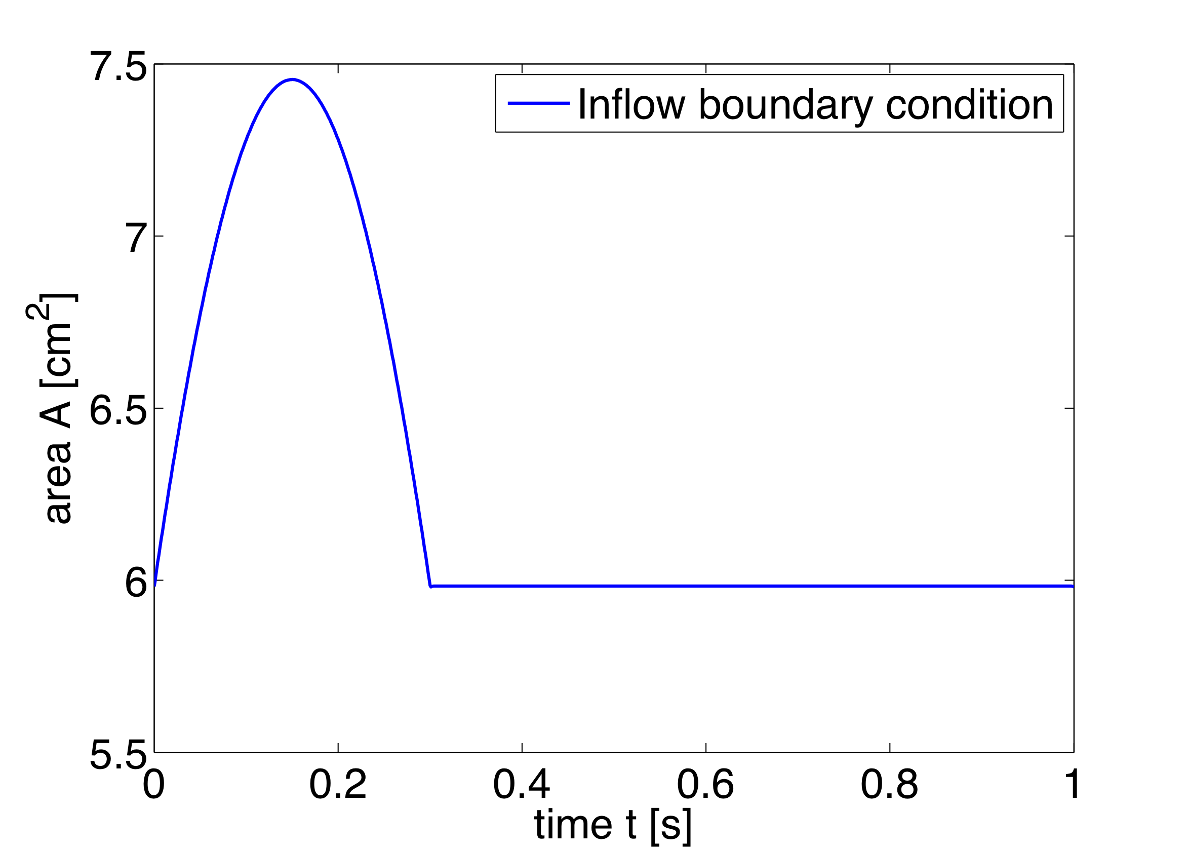
In the boundary conditions section the inflow and outflow conditions are set up. Here we use an inflow boundary condition for the area at the beginning of the ascending aorta taken from [30] and plotted on the right. Potential choices for inflow boundary conditions include Q-Inflow and Time-Dependent inflow. The outflow conditions for the terminal regions of the network could be specified by different models including eTerminal, R, CR, RCR and Time-Dependant outflow.

1<BOUNDARYCONDITIONS> 
2    <REGION REF="0"> <!-- Inflow --> 
3        <D VAR="A" USERDEFINEDTYPE="TimeDependent" 
4           VALUE="5.983*(1+0.597*(sin(6.28*t + 0.628) - 0.588)* 
5                (1./(1+exp(-2*200*(sin(6.28*t + 0.628) - 0.588)))))" /> 
6        <D VAR="u" USERDEFINEDTYPE="TimeDependent" VALUE="0.0" /> 
7    </REGION> 
8    <REGION REF="1"> 
9        <D VAR="A" USERDEFINEDTYPE="TimeDependent"  VALUE="A6" /> 
10        <D VAR="u" USERDEFINEDTYPE="TimeDependent"  VALUE="0.0" /> 
11    </REGION> 
12    <REGION REF="2"> 
13        <D VAR="A" USERDEFINEDTYPE="TimeDependent"  VALUE="A8" /> 
14        <D VAR="u" USERDEFINEDTYPE="TimeDependent"  VALUE="0.0" /> 
15    </REGION> 
16    <REGION REF="3"> 
17        <D VAR="A" USERDEFINEDTYPE="TimeDependent"  VALUE="A10" /> 
18        <D VAR="u" USERDEFINEDTYPE="TimeDependent"  VALUE="0.0" /> 
19    </REGION> 
20    .... 
21    <REGION REF="28"> 
22        <D VAR="A" USERDEFINEDTYPE="TimeDependent"  VALUE="A55" /> 
23        <D VAR="u" USERDEFINEDTYPE="TimeDependent"  VALUE="0.0" /> 
24    </REGION> 
25</BOUNDARYCONDITIONS>

Again, for the initial conditions we start our simulation from static equilibrium conditions A = A0 and for u being initially at rest. The following lines show how we specify A0 and β for different arterial segments.

1<FUNCTION NAME="InitialConditions"> 
2    <E VAR="A" DOMAIN="0" VALUE="5.983" /> 
3    <E VAR="u" DOMAIN="0" VALUE="0.0" /> 
4</FUNCTION> 
5   ... 
6<FUNCTION NAME="InitialConditions"> 
7    <E VAR="A" DOMAIN="54" VALUE="A55" /> 
8    <E VAR="u" DOMAIN="54" VALUE="0.0" /> 
9</FUNCTION> 
10 
11<FUNCTION NAME="A_0"> 
12    <E VAR="A_0" DOMAIN="0" VALUE="A1" /> 
13       ... 
14    <E VAR="A_0" DOMAIN="54" VALUE="A55" /> 
15</FUNCTION> 
16 
17<FUNCTION NAME="MaterialProperties"> 
18    <E VAR="beta" DOMAIN="0" VALUE="97" /> 
19      ... 
20    <E VAR="beta" DOMAIN="54" VALUE="9243" /> 
21</FUNCTION>

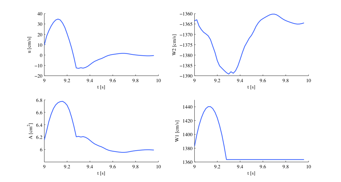
Our simulation is started as described before and the results show the time history for the conservative variables A and u, as well as for the characteristic variables W1 and W2 at the beginning of the ascending aorta (Artery 1). We can see that physically correct the shape of the inflow boundary condition appears in the forward traveling characteristic W1. As we do not have a terminal resistance at the outflow, one would normally expect W2 to be constant. However this is not the case, as bifurcations cause reflections if the radii of parent and daughter vessels are not well matching, leading to changes in W2. The shapes of A and u result from this facts and show the values for the physiological variables during one cardiac cycle. We may annotate that this values slightly differ from in vivo measurements due to the missing terminal resistance, which will be added in future.


PIC


These short examples should give an insight to the functionality of our PulseWaveSolver and show that results such as luminal area and pressure within the artery can be simulated. These results can contribute to understanding the physiology of the human vascular system and they can be used for patient-specific planning of medical interventions.

12.4.2 Stented Artery

12.4.3 Stented Artery

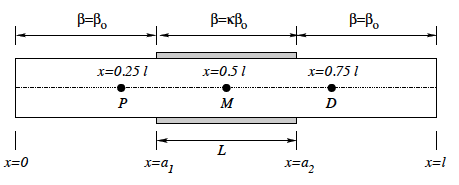
In the following we will explain the usage of the ?? to model the flow and pressure variation through a stented artery - a cardiovascular procedure in which a small mesh tube is inserted into an artery to restore blood flow through a constricted region. Due to the implantation of the stent this region will have different material properties compared to the the surrounding unstented tissue; hence will influence the propagation of waves through this system. The stent scenario to be modelled is a straight arterial segment with a stent situated between x = a1 and x = a2 as shown below.


PIC

Figure 12.2: Model of straight artery with a stent in the middle.


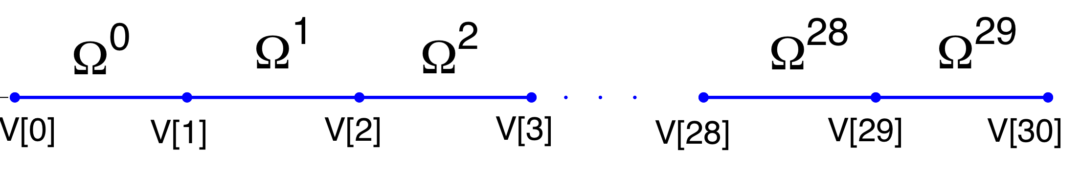
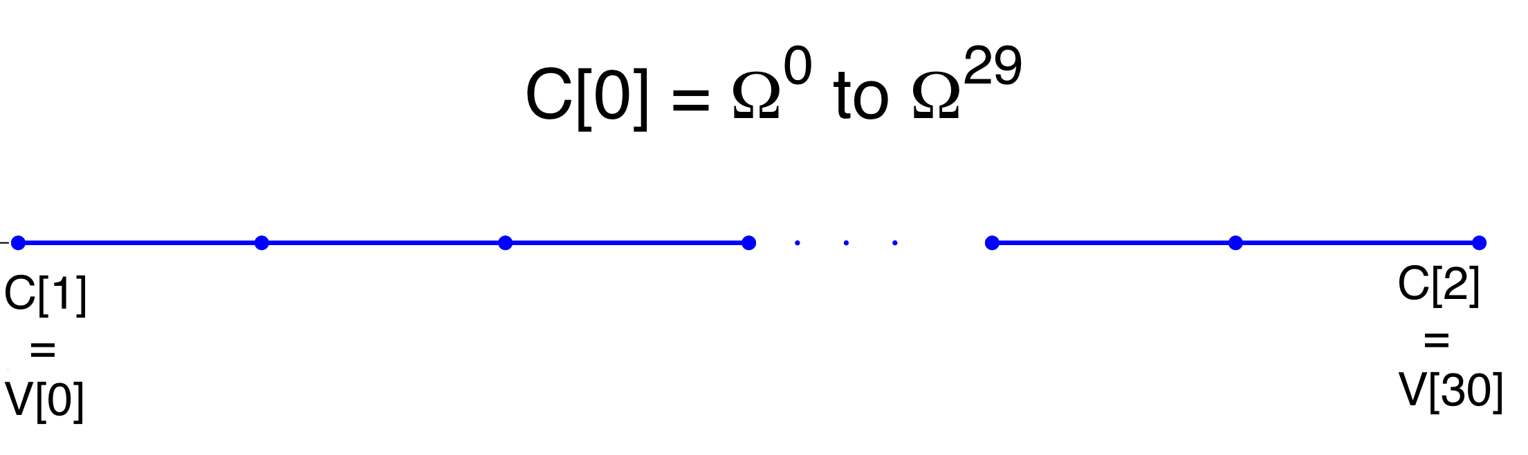
Geometry:  In the following we describe the geometry setup for modelling 1D flow in a stent. This is done by defining vertices, elements and composites. The vertices of the domain are shown below, consisting of 30 elements (Ω) and 31 vertices (V[n]).


PIC

Figure 12.3: 1D arterial domain consisting of 30 elements and 31 vertices.


To represent the above in the xml file, we define 31 vertices as follows:

1<VERTEX> 
2  <V ID="0"> 0.000e+00 0.000e+00 0.000e+00</V> 
3               . 
4               . 
5               . 
6  <V ID="30">30.000e+00 0.000e+00 0.000e+00</V> 
7</VERTEX>

and the connectivity of these vertices to make up the 30 elements:

1<ELEMENT> 
2  <S ID="0">    0     1 </S> 
3               . 
4               . 
5               . 
6  <S ID="29">   29    30 </S> 
7</ELEMENT>

These elements are combined to three different composites (shown below): composite 0 represents all the elements; composite 1 the inflow boundary and composite 2 the outflow boundary.


PIC

Figure 12.4: Three composites (C[0], C[1] and C[2]) for the stunted artery.


The above composites are specified as follows:

1<COMPOSITE> 
2  <C ID="0"> S[0-29] </C> 
3  <C ID="1"> V[0] </C> 
4  <C ID="2"> V[30] </C> 
5</COMPOSITE>

Finally the domain is specified by the first composite by

1<DOMAIN> 
2  <D ID="0"> C[0] </D> 
3</DOMAIN>

Expansion:  For the expansions we use 4th-order polynomials which define our two variables A and u on the domain.

1<EXPANSIONS> 
2  <E COMPOSITE="C[0]" NUMMODES="5" FIELDS="A,u" TYPE="MODIFIED" /> 
3</EXPANSIONS>

Solver Information:  The Discontinuous Galerkin Method is used as projection scheme and the time-integration is performed by a simple Forward Euler scheme. A full list of possible time integration scheme is given in the parameter section of the ??

1<SOLVERINFO> 
2  <I PROPERTY="EQTYPE" VALUE="PulseWavePropagation" /> 
3  <I PROPERTY="Projection" VALUE="DisContinuous" /> 
4  <I PROPERTY="TimeIntegrationMethod" VALUE="ForwardEuler" /> 
5  <I PROPERTY="UpwindTypePulse"  VALUE="UpwindPulse"/> 
6</SOLVERINFO>

Parameters:  Parameters used for the simulation are taken from [30]

1<PARAMETERS> 
2   <P> TimeStep       = 2e-6               </P> 
3   <P> FinTime        = 0.25               </P> 
4   <P> NumSteps       = FinTime/TimeStep   </P> 
5   <P> IO_CheckSteps  = NumSteps/50        </P> 
6   <P> IO_InfoSteps   = 100                </P> 
7   <P> T              = 0.33               </P> 
8   <P> h0             = 1.0                </P> 
9   <P> rho            = 1.0                </P> 
10   <P> nue            = 0.5                </P> 
11   <P> pext           = 0.0                </P> 
12   <P> a1             = 10.0               </P> 
13   <P> a2             = 20.0               </P> 
14   <P> kappa          = 100.0              </P> 
15   <P> Y0             = 1.9099e+5          </P> 
16   <P> k              = 2                  </P> 
17   <P> k1             = 200                </P> 
18 </PARAMETERS>

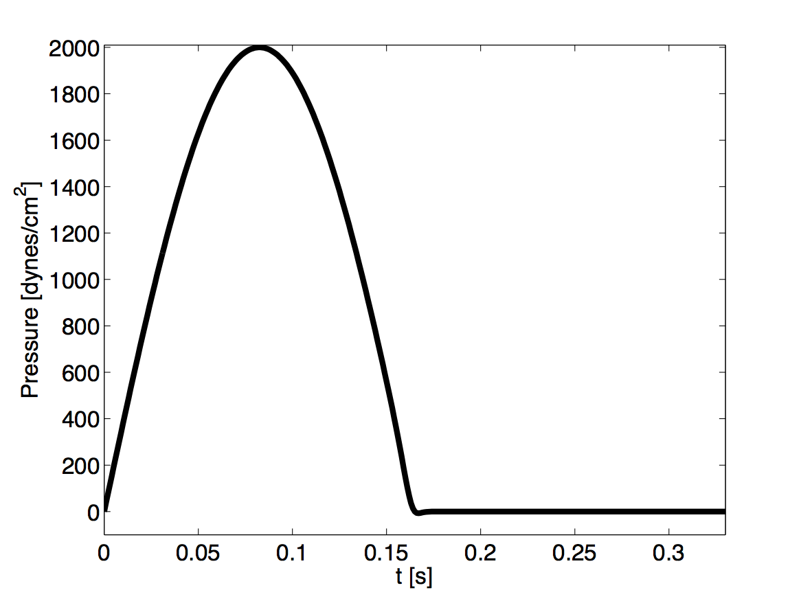
Boundary conditions:  At the inflow we apply a pressure boundary condition as shown in the figure below. This condition models the pressure variation during one heartbeat. A simple absorbing outflow boundary condition is applied the right end of the tube.


PIC

Figure 12.5: Pressure profile applied at the inlet of the artery


These are defined in the xml file as follows,

1<BOUNDARYREGIONS> 
2   <B ID="0"> C[1] </B> 
3   <B ID="1"> C[2] </B> 
4</BOUNDARYREGIONS> 
5 
6<BOUNDARYCONDITIONS> 
7   <REGION REF="0"> 
8      <D VAR="A" USERDEFINEDTYPE="TimeDependent" VALUE= 
9      "(2000*sin(2*PI*t/T)*1./(1+exp(-2*k1*(T/2-t))-pext)/451352+1)^2" /> 
10      <D VAR="u" USERDEFINEDTYPE="TimeDependent" VALUE="1.0" /> 
11   </REGION> 
12   <REGION REF="1"> 
13      <D VAR="A" VALUE="1.0" /> 
14      <D VAR="u" VALUE="1.0" /> 
15   </REGION> 
16</BOUNDARYCONDITIONS>

The simulation starts from the static equilibrium of the vessel with normalised area and velocity.

1<FUNCTION NAME="InitialConditions"> 
2        <E VAR="A" DOMAIN="0" VALUE="1.0" /> 
3        <E VAR="u" DOMAIN="0" VALUE="1.0" /> 
4</FUNCTION> 
5 
6<FUNCTION NAME="A_0"> 
7        <E VAR="A" DOMAIN="0" VALUE="1.0" /> 
8</FUNCTION>

Functions:  The stent is introduced by applying a variable material properties function (β - see equation 12.2) along the vessel in the x direction, shown graphically below


PIC

Figure 12.6: material property variation along the artery. The stiff region in the middle represents the stent.


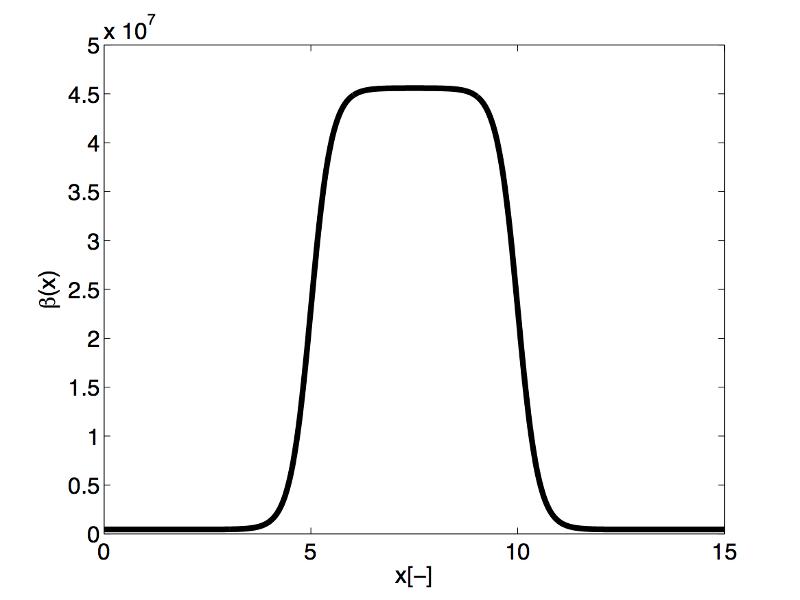
and defined in the xml file by

1<FUNCTION NAME="MaterialProperties"> 
2        <E VAR="E0" DOMAIN="0" VALUE= 
3        "Y0*(1.0-kappa/(1+exp(-2*k*(a1-x)))+kappa/(1+exp(-2*k*(a2-x))))" /> 
4</FUNCTION>
12.4.3.1 Simulation

The simulation is started by running

PulseWaveSolver Test_1.xml

It will take about 60 seconds on a 2.4GHz Intel Core 2 Duo processor and therefore is computationally realisable at every clinical site.

12.4.3.2 Results

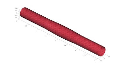
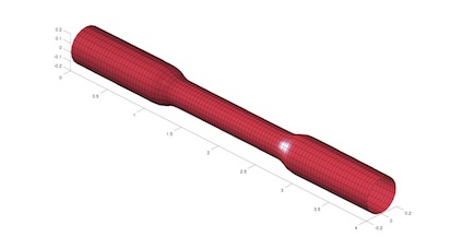
As a result we get a 3-dimensional interpretation of the aortic cross-sectional area varying in axial direction both for the stented and non-stented vessel. In case of the stent, the rigid metal mesh will restrict the deformation of the area in that specific part of the artery compared to the normal vessel (Fig. 12.7).


PIC PIC

Figure 12.7:


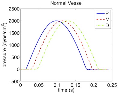
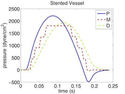
Also, if we look at the pressure at three points within the artery (P, M, D) we will recognize that there are major differences between the stented and normal vessel. While in the normal vessel (left) the pressure wave applied at the inflow is propagated without any losses, this does not hold for the stented artery (right). Here, the stiffening at the stent causes reflections and thus there are losses for total pressure at the medial (M) and distal (D) point.


PIC PIC