13.1 Synopsis

The ShallowWaterSolver is a solver for depth-integrated wave equations of shallow water type. Presently the following equations are supported:

13.1.1 The Shallow Water Equations

The shallow water equations (SWE) is a two-dimensional system of nonlinear partial differential equations of hyperbolic type that are fundamental in hydraulic, coastal and environmental engineering. In deriving the SWE the vertical velocity is considered negligible and the horizontal velocities are assumed uniform with depth. The SWE are hence valid when the water depth can be considered small compared to the characteristic length scale of the problem, as typical for flows in rivers and shallow coastal areas. Despite the limiting restrictions the SWE can be used to describe many important phenomena, for example storm surges, tsunamis and river flooding.

The two-dimensional SWE is stated in conservation form as

+ ∇⋅F(U) = S(U)

where F(U) = is the flux vector and the vector of conserved variables read U = ^T. Here H(x,t) = ζ(x,t) + d(x) is the total water depth, ζ(x,t) is the free surface elevation and d(x) is the still water depth. The depth-averaged velocity is denoted by u(x,t) = ^T, where u and v are the velocities in the x- and y-directions, respectively. The content of the flux vector is

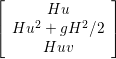E(U) = , G(U) = ,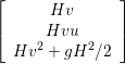

in which g is the acceleration due to gravity. The source term S(U) accounts for, e.g., forcing due to bed friction, bed slope, Coriolis force and higher-order dispersive effects (Boussinesq terms). In the distributed version of the ShallowWaterSolver only the Coriolis force is included.