9.4 Examples

9.4.1 Shock capturing

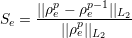
Compressible flow is characterised by abrupt changes in density within the flow domain often referred to as shocks. These discontinuities lead to numerical instabilities (Gibbs phenomena). This problem is prevented by locally adding a diffusion term to the equations to damp the numerical fluctuations. These fluctuations in an element are identified using a sensor algorithm which quantifies the smoothness of the solution within an element. The value of the sensor in an element is defined as

(9.8)

An artificial diffusion term is introduced locally to the Euler equations to deal with flow discontinuity and the consequential numerical oscillations. Two models are implemented, a non-smooth and a smooth artificial viscosity model.

9.4.1.1 Non-smooth artificial viscosity model

For the non-smooth artificial viscosity model the added artificial viscosity is constant in each element and discontinuous between the elements. The Euler system is augmented by an added laplacian term on right hand side of equation 9.1. The diffusivity of the system is controlled by a variable viscosity coefficient ϵ. The value of ϵ is dependent on ϵ₀, which is the maximum viscosity that is dependent on the polynomial order (p), the mesh size (h) and the maximum wave speed and the local sensor value. Based on pre-defined sensor threshold values, the variable viscosity is set accordingly

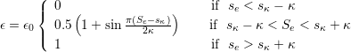(9.9)

To enable the non-smooth viscosity model, the following line has to be added to the SOLVERINFO section:

The diffusivity is controlled by the following parameters:

where mu0 is the maximum values for the viscosity coefficient, Kappa is half of the width of the transition interval and Skappa is the value of the centre of the interval.

9.4.1.2 Smooth artificial viscosity model

For the smooth artificial viscosity model an extra PDE for the artificial viscosity is appended to the Euler system

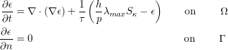(9.10)

where S_κ is a normalised sensor value and serves as a forcing term for the artificial viscosity. A smooth artificial viscosity distribution is obtained.

To enable the smooth viscosity model, the following line has to be added to the SOLVERINFO section:

Furthermore, the extra viscosity variable eps has to be added to the variable list:

A similar addition has to be made for the boundary conditions and initial conditions. The tests that have been run started with a uniform homogeneous boundary condition and initial condition. The following parameters can be set in the xml session file:

where for now FH and FL are used to tune which range of the sensor is used as a forcing term and C1 and C2 are fixed constants which can be played around with to make the model more diffusive or not. However these constants are generally fixed.

9.4.2 Variable polynomial order

A sensor based p-adaptive algorithm is implemented to optimise the computational cost and accuracy. The DG scheme allows one to use different polynomial orders since the fluxes over the elements are determined using a Riemann solver and there is now further coupling between the elements. Furthermore, the initial p-adaptive algorithm uses the same sensor as the shock capturing algorithm to identify the smoothness of the local solution so it rather straightforward to implement both algorithms at the same time.

The polynomial order in each element can be adjusted based on the sensor value that is obtained. Initially, a converged solution is obtained after which the sensor in each element is calculated. Based on the determined sensor value and the pre-defined sensor thresholds, it is decided to increase, decrease or maintain the degree of the polynomial approximation in each element and a new converged solution is obtained.

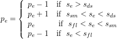(9.11)

For now, the threshold values s_e, s_ds, s_sm and s_fl are determined empirically by looking at the sensor distribution in the domain. Once these values are set, two .txt files are outputted, one that has the composites called VariablePComposites.txt and one with the expansions called VariablePExpansions.txt. These values have to copied into a new .xml file to create the adapted mesh.

9.4.3 De-Aliasing Techniques

Aliasing effects, arising as a consequence of the nonlinearity of the underlying problem, need to be address to stabilise the simulations. Aliasing appears when nonlinear quantities are calculated at an insufficient number of quadrature points. We can identify two types of nonlinearities:

• PDE nonlinearities, related to the nonlinear and quasi-linear fluxes.
• Geometrical nonlinearities, related to the deformed/curves meshes.

We consider two de-aliasing strategies based on the concept of consistent integration:

• Local dealiasing: It only targets the PDE-aliasing sources, applying a consistent integration of them locally.
• Global dealiasing: It targets both the PDE and the geometrical-aliasing sources. It requires a richer quadrature order to consistently integrate the nonlinear fluxes, the geometric factors, the mass matrix and the boundary term.

Since Nektar++ tackles separately the PDE and geometric aliasing during the projection and solution of the equations, to consistently integrate all the nonlinearities in the compressible NavierStokes equations, the quadrature points should be selected based on the maximum order of the nonlinearities:

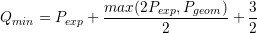(9.12)

where Q_min is the minimum required number of quadrature points to exactly integrate the highest-degree of nonlinearity, P_exp being the order of the polynomial expansion and P_geom being the geometric order of the mesh. Bear in mind thatwe are using a discontinuous discretisation, meaning that aliasing effect are not fully controlled, since the boundary terms introduce non-polynomial functions into the problem.

To enable the global de-aliasing technique, modify the number of quadrature points by:

where NUMMODES corresponds to P+1, where P is the order of the polynomial used to approximate the solution. NUMPOINTS specifies the number of quadrature points.