 . Hence, they describe the evolution of perturbations
 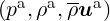 around this state. In conservative form, the LEE are given as:
The aim of the AcousticSolver is to predict acoustic wave propagation. Through the application of a splitting technique, the flow-induced acoustic field is totally decoupled from the underlying hydrodynamic field.
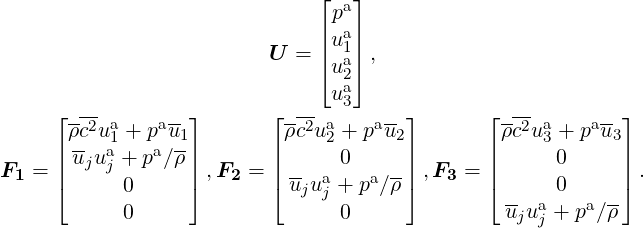
The Linearized Euler Equations (LEE) are obtained by linearizing the Euler Equations about
a mean flow state . Hence, they describe the evolution of perturbations
around this state. In conservative form, the LEE are given as:
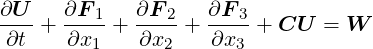 | (6.1) |
with
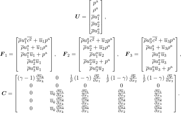 | (6.2) (6.3) (6.4) |
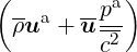
The acoustic perturbation equations (APE-1/APE-4) proposed by Ewert and Schroeder [13] assure stable aeroacoustic simulations. These equations are similar to the LEE, but account for acoustic perturbations exclusively. The AcousticSolver implements the APE-1/4 type operator:
where (u,c2,ρ) represents the base flow and (ua,pa) the acoustic perturbations. Similar to the
LEE, the acoustic source terms  c and
c and  m are by default zero and must be specified e.g. by an
appropriate forcing. This way, e.g. the APE-1, APE-4 [13] or revised APE equations [15]
can be obtained. Expressed as hyperbolic conservation law, the APE-1/4 operator
reads:
m are by default zero and must be specified e.g. by an
appropriate forcing. This way, e.g. the APE-1, APE-4 [13] or revised APE equations [15]
can be obtained. Expressed as hyperbolic conservation law, the APE-1/4 operator
reads:
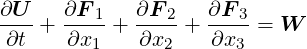 | (6.6) |
with
 | (6.7) (6.8) |
 +
+
 c
c + ∇
+ ∇ + ∇
+ ∇
 m,
m,