6.4 Examples
6.4.1 Wave Propagation in a Sheared Base Flow
In this section we explain how to set up a simple, 2D simulation of aeroacoustics in Nektar++.
We will study the propagation of an acoustic wave in the simple case of a sheared base flow,
i.e. u = ![[300tanh(20x2),0]](user-guide42x.png) T,c2 =
T,c2 =  2,ρ = 1.204kg∕m3. The geometry consists of 64
quadrilateral elements.
2,ρ = 1.204kg∕m3. The geometry consists of 64
quadrilateral elements.
6.4.1.1 Input file
We require a discontinuous Galerkin projection and use an explicit fourth-order
Runge-Kutta time integration scheme. We therefore set the following solver information:
1<SOLVERINFO>
2 <I PROPERTY="EQType" VALUE="APE"/>
3 <I PROPERTY="Projection" VALUE="DisContinuous"/>
4 <I PROPERTY="TimeIntegrationMethod" VALUE="ClassicalRungeKutta4"/>
5 <I PROPERTY="UpwindType" VALUE="LaxFriedrichs"/>
6</SOLVERINFO>
To maintain numerical stability we must use a small time-step. Finally, we set the density,
heat ratio and ambient pressure.
1<PARAMETERS>
2 <P> TimeStep = 1e-05 </P>
3 <P> NumSteps = 1000 </P>
4 <P> FinTime = TimeStep*NumSteps </P>
5 <P> IO_CheckSteps = 10 </P>
6 <P> IO_InfoSteps = 10 </P>
7</PARAMETERS>
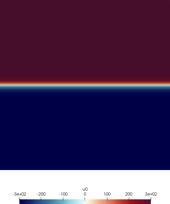
The initial condition and the base flow field are specified by the Baseflow and
InitialConditions functions, respectively:
1<FUNCTION NAME="Baseflow">
2 <E VAR="u0" VALUE="300 * tanh(2*y/0.1)"/>
3 <E VAR="v0" VALUE="0"/>
4 <E VAR="c0sq" VALUE="1.4 * Pinfinity / Rho0"/>
5 <E VAR="rho0" VALUE="Rho0"/>
6</FUNCTION>
7<FUNCTION NAME="InitialConditions">
8 <E VAR="p" VALUE="0"/>
9 <E VAR="u" VALUE="0"/>
10 <E VAR="v" VALUE="0"/>
11</FUNCTION>
At all four boundaries the RiemannInvariantBC condition is used:
1<BOUNDARYCONDITIONS>
2 <REGION REF="0">
3 <D VAR="p" USERDEFINEDTYPE="RiemannInvariantBC"/>
4 <D VAR="u" USERDEFINEDTYPE="RiemannInvariantBC"/>
5 <D VAR="v" USERDEFINEDTYPE="RiemannInvariantBC"/>
6 </REGION>
7</BOUNDARYCONDITIONS>
The system is excited via an acoustic source term  c, which is modeled by a field forcing as:
1<FORCING>
2 <FORCE TYPE="Field">
3 <FIELDFORCE> Source <FIELDFORCE/>
4 </FORCE>
5</FORCING>
and the corresponding function
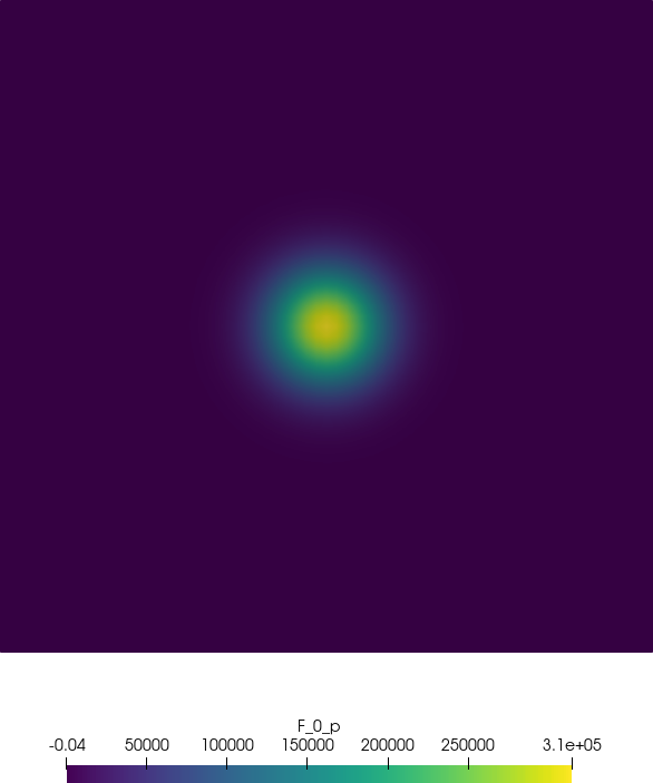
1<FUNCTION NAME="Source">
2 <E VAR="p" VALUE="100 * 2*PI*5E2 * cos(2*PI*5E2 * t) * exp(-32*(x^2+y^2))"/>
3 <E VAR="u" VALUE="0"/>
4 <E VAR="v" VALUE="0"/>
5</FUNCTION>
6.4.1.2 Running the code
AcousticSolver Test_pulse.xml
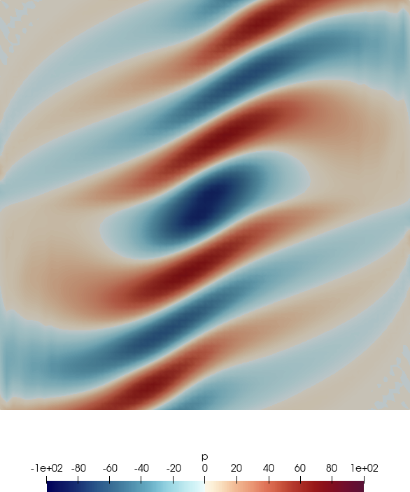
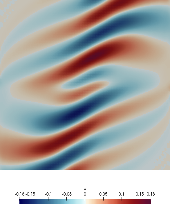
6.4.1.3 Results
Fig. 6.1 shows the acoustic source term, the velocity and the acoustic pressure and velocity
perturbations at a single time step.