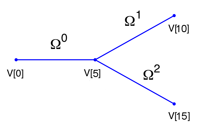
Typically 1D arterial networks are made up of a connection of different base units: segments, bifurcations and merging junctions. The input format in the PulseWaveSolver means these connections are handle naturally from the mesh topology; hence care must be taken when designing the 1D domain. The figure below outlines the structure of a bifurcation, which is a common reoccurring structure in the vasculature.

To represent this topology in the xml file we specify the following vertices under the section
VERTEX (the extents are: -100 ≥ x ≤ 100 and -100 ≥ y ≤ 100 )
The elements from these vertices are then constructed under the section ELEMENT by defining
The composites, which represent groups of elements and boundary regions are defined under
the section COMPOSITE by
Each of the segments can be then represented under the section DOMAIN by
We will use the different domains later to define variable material properties and cross-sectional areas.
The PulseWaveSolver is sqpecified through the EquationType option in the session file. This
can be set as follows:
Projection: Only a discontinuous projection can be specified using the following
option:
Discontinuous for a discontinous Galerkin (DG) projection.TimeIntegrationMethod
UpwindTypePulse:
UpwindPulse
The following parameters can be specified in the PARAMETERS section of the session file.
TimeStep is the time-step size;
FinTime is the final physical time at which the simulation will stop;
NumSteps is the equivalent of FinTime but instead of specifying the physical final
time the number of time-steps is defined;
IO_CheckSteps sets the number of steps between successive checkpoint files;
IO_InfoSteps sets the number of steps between successive info stats are printed
to screen;
rho density of the fluid. Default value = 1.0;
nue Poisson’s ratio. Default value = 0.5 ;
pest external pressure. Default value = 0;
h0 wall thickness Default value = 1.0;
In this section we can specify the boundary conditions for our problem. First we need to define
the variables under the section VARIABLES.
The composites that we want to apply out boundary conditions then need to be defined
in the BOUNDARYREGIONS, for example if we had three composites (C[1], C[4] and
C[8]) that correspond to three vertices of the computational mesh we would define:
Finally we can specify the boundary conditions on the regions specified under
BOUNDARYREGIONS.
The Pulse Wave Solver comes with a number of boundary conditions that are unique to this solver. Boundary conditions must be provided for both the area and velocity at the inlets and outlets of the domain. Examples of the different boundary conditions will be provided in the following.
Inlet boundary condition:
The inlet condition may be specified algebraically in four different ways: as an area
variation (A-inflow); a velocity profile (U-inflow); a volume flux (Q-inflow); or by
prescribing the forward characteristic (TimeDependent). When prescribing a volume flux,
it must be specified in the input file via the area, as illustrated below. Note that
u = 1.0.
Terminal boundary conditions:
At the outlets of the domain there are four possible boundary conditions: reflection
(Terminal), terminal resistance R-terminal, Two element windkessel (CR) CR-terminal, and
three element windkessel (RCR) RCR-terminal. An example of the outflow boundary
condition of the RCR terminal is given below
Where RT is the total peripheral resistance used in the the R-terminal, CR-terminal and
RCR-terminal models
The following functions can be specified inside the CONDITIONS section of the session file:
MaterialProperties: specifies the material properties for each domain.
A_0: Initial area of each domain.
AdvectionVelocity: specifies the advection velocity v.
InitialConditions: specifies the initial condition for unsteady problems.
Forcing: specifies the forcing function fAs an example to specify the material properties for each domain in the previous bifurcation example we would enter:
The values of beta are used in the pressure-area relationship (equation 13.2).