3.4 Filters
Filters are a method for calculating a variety of useful quantities from the field variables as the
solution evolves in time, such as time-averaged fields and extracting the field variables at
certain points inside the domain. Each filter is defined in a FILTER tag inside a
FILTERS block which lies in the main NEKTAR tag. In this section we give an overview
of the modules currently available and how to set up these filters in the session
file.
Here is an example FILTER:
1<FILTER TYPE="FilterName">
2 <PARAM NAME="Param1"> Value1 </PARAM>
3 <PARAM NAME="Param2"> Value2 </PARAM>
4</FILTER>
A filter has a name – in this case, FilterName – together with parameters which are set to
user-defined values. Each filter expects different parameter inputs, although where
functionality is similar, the same parameter names are shared between filter types for
consistency. Numerical filter parameters may be expressions and so may include session
parameters defined in the PARAMETERS section.
Some filters may perform a large number of operations, potentially taking up a
significant percentage of the total simulation time. For this purpose, the parameter
IO_FiltersInfoSteps is used to set the number of steps between successive total filter CPU
time stats are printed. By default it is set to 10 times IO_InfoSteps. If the solver is run with
the verbose -v flag, further information is printed, detailing the CPU time of each individual
filter and percentage of time integration.
In the following we document the filters implemented. Note that some filters are solver-specific
and will therefore only work for a given subset of the available solvers.
3.4.1 Phase sampling
Note: This feature is currently only supported for filters derived from the FieldConvert filter:
AverageFields, MovingAverage, ReynoldsStresses.
When analysing certain time-dependent problems, it might be of interest to activate a filter in
a specific physical phase and with a certain period (for instance, to carry out phase averaging).
The simulation time can be written as t = mT + nT T , where m is an integer representing the
number of periods T elapsed, and 0 ≤ nT ≤ 1 is the phase. This feature is not a
filter in itself and it is activated by adding the parameters below to the filter of
interest:
| Option name | Required | Default | Description
|
PhaseAverage | ✓ | | Feature activation
|
PhaseAveragePeriod | ✓ | | Period T
|
PhaseAveragePhase | ✓ | | Phase nT .
|
| |
For instance, to activate phase averaging with a period of T = 10 at phase nT = 0.5:
1<FILTER TYPE="FilterName">
2 <PARAM NAME="Param1"> Value1 </PARAM>
3 <PARAM NAME="Param2"> Value2 </PARAM>
4 <PARAM NAME="PhaseAverage"> True </PARAM>
5 <PARAM NAME="PhaseAveragePeriod"> 10 </PARAM>
6 <PARAM NAME="PhaseAveragePhase"> 0.5 </PARAM>
7</FILTER>
Since this feature monitors nT every SampleFrequency, for best results it is recommended to
set SampleFrequency= 1.
The maximum error in sampling phase is nT ,tol =  ⋅
⋅ SampleFrequency, which is
displayed at the beginning of the simulation if the solver is run with the verbose -v
option.
The number of periods elapsed is calculated based on simulation time. Caution is therefore
recommended when modifying time information in the restart field, because if the new
time does not correspond to the same phase, the feature will produce erroneous
results.
3.4.2 Aerodynamic forces
Note: This filter is only supported for the incompressible Navier-Stokes solver.
This filter evaluates the aerodynamic forces along a specific surface. The forces are projected
along the Cartesian axes and the pressure and viscous contributions are computed in each
direction.
The following parameters are supported:
| Option name | Required | Default | Description
|
OutputFile | ✗ | session | Prefix of the output filename to
which the forces are written.
|
Frequency | ✗ | 1 | Number of timesteps after which
output is written.
|
Boundary | ✓ | - | Boundary surfaces on which the
forces are to be evaluated.
|
| |
An example is given below:
1 <FILTER TYPE="AeroForces">
2 <PARAM NAME="OutputFile">DragLift</PARAM>
3 <PARAM NAME="OutputFrequency">10</PARAM>
4 <PARAM NAME="Boundary"> B[1,2] </PARAM>
5 </FILTER>
During the execution a file named DragLift.fce will be created and the value of the
aerodynamic forces on boundaries 1 and 2, defined in the GEOMETRY section, will be output
every 10 time steps.
3.4.3 Benchmark
Note: This filter is only supported for the Cardiac Electrophysiology Solver.
Filter Benchmark records spatially distributed event times for activation and repolarisation
(recovert) during a simulation, for undertaking benchmark test problems.
1<FILTER TYPE="Benchmark">
2 <PARAM NAME="ThresholdValue"> -40.0 </PARAM>
3 <PARAM NAME="InitialValue"> 0.0 </PARAM>
4 <PARAM NAME="OutputFile"> benchmark </PARAM>
5 <PARAM NAME="StartTime"> 0.0 </PARAM>
6</FILTER>
ThresholdValue specifies the value above which tissue is considered to be
depolarised and below which is considered repolarised.
InitialValue specifies the initial value of the activation or repolarisation time
map.
OutputFile specifies the base filename of activation and repolarisation maps
output from the filter. This name is appended with the index of the event and the
suffix ‘.fld‘.
StartTime (optional) specifies the simulation time at which to start detecting
events.
3.4.4 Cell history points
Note: This filter is only supported for the Cardiac Electrophysiology Solver.
Filter CellHistoryPoints writes all cell model states over time at fixed points. Can be used
along with the HistoryPoints filter to record all variables at specific points during a
simulation.
1<FILTER TYPE="CellHistoryPoints">
2 <PARAM NAME="OutputFile">crn.his</PARAM>
3 <PARAM NAME="OutputFrequency">1</PARAM>
4 <PARAM NAME="Points">
5 0.00 0.0 0.0
6 </PARAM>
7</FILTER>
OutputFile specifies the filename to write history data to.
OutputFrequency specifies the number of steps between successive outputs.
Points lists coordinates at which history data is to be recorded.
3.4.5 Checkpoint cell model
Note: This filter is only supported for the Cardiac Electrophysiology Solver.
Filter CheckpointCellModel checkpoints the cell model. Can be used along with
the Checkpoint filter to record complete simulation state and regular intervals.
1<FILTER TYPE="CheckpointCellModel">
2 <PARAM NAME="OutputFile"> session </PARAM>
3 <PARAM NAME="OutputFrequency"> 1 </PARAM>
4</FILTER>
OutputFile (optional) specifies the base filename to use. If not specified, the
session name is used. Checkpoint files are suffixed with the process ID and the
extension ‘.chk‘.
OutputFrequency specifies the number of timesteps between checkpoints.
3.4.6 Checkpoint fields
The checkpoint filter writes a checkpoint file, containing the instantaneous state of the
solution fields at at given timestep. This can subsequently be used for restarting the
simulation or examining time-dependent behaviour. This produces a sequence of files, by
default named session_*.chk, where * is replaced by a counter. The initial condition is
written to session_0.chk. Existing files are not overwritten, but renamed to e.g.
session_0.bak0.chk. In case this file already exists, too, the chk-file is renamed to
session_0.bak*.chk and so on.
Note: This functionality is equivalent to setting the IO_CheckSteps parameter in the session
file.
The following parameters are supported:
| Option name | Required | Default | Description
|
OutputFile | ✗ | session | Prefix of the output filename
to which the checkpoints are
written.
|
OutputFrequency | ✓ | - | Number of timesteps after
which output is written.
|
| |
For example, to output the fields every 100 timesteps we can specify:
1<FILTER TYPE="Checkpoint">
2 <PARAM NAME="OutputFile">IntermediateFields</PARAM>
3 <PARAM NAME="OutputFrequency">100</PARAM>
4</FILTER>
3.4.7 Electrogram
Note: This filter is only supported for the Cardiac Electrophysiology Solver.
Filter Electrogram computes virtual unipolar electrograms at a prescribed set of points.
1<FILTER TYPE="Electrogram">
2 <PARAM NAME="OutputFile"> session </PARAM>
3 <PARAM NAME="OutputFrequency"> 1 </PARAM>
4 <PARAM NAME="Points">
5 0.0 0.5 0.7
6 1.0 0.5 0.7
7 2.0 0.5 0.7
8 </PARAM>
9</FILTER>
OutputFile (optional) specifies the base filename to use. If not specified, the
session name is used. The extension ‘.ecg‘ is appended if not already specified.
OutputFrequency specifies the number of resolution of the electrogram data.
Points specifies a list of coordinates at which electrograms are desired. They must
not lie within the domain.
3.4.8 FieldConvert checkpoints
This filter applies a sequence of FieldConvert modules to the solution, writing an output file.
An output is produced at the end of the simulation into session_fc.fld, or alternatively
every M timesteps as defined by the user, into a sequence of files session_*_fc.fld, where *
is replaced by a counter.
Module options are specified as a colon-separated list, following the same syntax as the
FieldConvert command-line utility (see Section 5).
The following parameters are supported:
| Option name | Required | Default | Description
|
OutputFile | ✗ | session.fld | Output filename. If no
extension is provided, it
is assumed as .fld
|
OutputFrequency | ✗ | NumSteps | Number
of timesteps after which
output is written, M.
|
Modules | ✗ | | FieldConvert modules to
run, separated by a white
space.
|
| |
As an example, consider:
1<FILTER TYPE="FieldConvert">
2 <PARAM NAME="OutputFile">MyFile.vtu</PARAM>
3 <PARAM NAME="OutputFrequency">100</PARAM>
4 <PARAM NAME="Modules"> vorticity isocontour:fieldid=0:fieldvalue=0.1 </PARAM>
5</FILTER>
This will create a sequence of files named MyFile_*_fc.vtu containing isocontours. The result
will be output every 100 time steps.
3.4.9 History points
The history points filter can be used to evaluate the value of the fields in specific points of the
domain as the solution evolves in time. By default this produces a file called session.his. For
each timestep, and then each history point, a line is output containing the current solution
time, followed by the value of each of the field variables. Commented lines are created at the
top of the file containing the location of the history points and the order of the
variables.
The following parameters are supported:
| Option name | Required | Default | Description
|
OutputFile | ✗ | session | Prefix of the output filename
to which the checkpoints are
written.
|
OutputFrequency | ✗ | 1 | Number of timesteps after
which output is written.
|
OutputPlane | ✗ | 0 | If the simulation
is homogeneous, the plane on
which
to evaluate the history point.
(No Fourier interpolation is
currently implemented.)
|
Points | ✓ | - | A list of the history points.
These should always be given
in three dimensions.
|
| |
For example, to output the value of the solution fields at three points (1,0.5,0),
(2,0.5,0) and (3,0.5,0) into a file TimeValues.his every 10 timesteps, we use the
syntax:
1<FILTER TYPE="HistoryPoints">
2 <PARAM NAME="OutputFile">TimeValues</PARAM>
3 <PARAM NAME="OutputFrequency">10</PARAM>
4 <PARAM NAME="Points">
5 1 0.5 0
6 2 0.5 0
7 3 0.5 0
8 </PARAM>
9</FILTER>
3.4.10 Kinetic energy and enstrophy
Note: This filter is only supported for the incompressible and compressible Navier-Stokes
solvers in three dimensions.
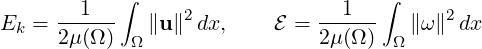
The purpose of this filter is to calculate the kinetic energy and enstrophy
where μ(Ω) is the volume of the domain Ω. This produces a file containing the time-evolution
of the kinetic energy and enstrophy fields. By default this file is called session.eny where
session is the session name.
The following parameters are supported:
| Option name | Required | Default | Description
|
OutputFile | ✗ | session.eny | Output file name
to which the energy and
enstrophy are written.
|
OutputFrequency | ✓ | - | Number of timesteps at
which output is written.
|
| |
To enable the filter, add the following to the FILTERS tag:
1<FILTER TYPE="Energy">
2 <PARAM NAME="OutputFrequency"> 1 </PARAM>
3</FILTER>
3.4.11 Modal energy
Note: This filter is only supported for the incompressible Navier-Stokes solver.
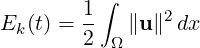
This filter calculates the time-evolution of the kinetic energy. In the case of a two- or
three-dimensional simulation this is defined as
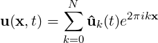
However if the simulation is written as a one-dimensional homogeneous expansion so
that
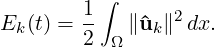
then we instead calculate the energy spectrum
Note that in this case, each component of ûk is a complex number and therefore
N = HomModesZ∕2 lines are output for each timestep. This is a particularly useful tool in
examining turbulent and transitional flows which use the homogeneous extension.
In either case, the resulting output is written into a file called session.mdl by
default.
The following parameters are supported:
| Option name | Required | Default | Description
|
OutputFile | ✗ | session | Prefix of the output filename
to which the energy spectrum
is written.
|
OutputFrequency | ✗ | 1 | Number of timesteps after
which output is written.
|
| |
An example syntax is given below:
1<FILTER TYPE="ModalEnergy">
2 <PARAM NAME="OutputFile">EnergyFile</PARAM>
3 <PARAM NAME="OutputFrequency">10</PARAM>
4</FILTER>
3.4.12 Moving body
Note: This filter is only supported for the Quasi-3D incompressible Navier-Stokes solver, in
conjunction with the MovingBody forcing.
This filter MovingBody is encapsulated in the forcing module to evaluate the aerodynamic
forces along the moving body surface. It is described in detail in section 11.3.4.1
3.4.13 Moving average of fields
This filter computes the exponential moving average (in time) of fields for each variable
defined in the session file. The moving average is defined as:
with 0 < α < 1 and u1 = u1.
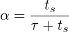
The same parameters of the time-average filter are supported, with the output file in the form
session_*_movAvg.fld. In addition, either α or the time-constant τ must be defined. They
are related by:
where ts is the time interval between consecutive samples.
As an example, consider:
1<FILTER TYPE="MovingAverage">
2 <PARAM NAME="OutputFile">MyMovingAverage</PARAM>
3 <PARAM NAME="OutputFrequency">100</PARAM>
4 <PARAM NAME="SampleFrequency"> 10 </PARAM>
5 <PARAM NAME="tau"> 0.1 </PARAM>
6</FILTER>
This will create a file named MyMovingAverage_movAvg.fld with a moving average
sampled every 10 time steps. The averaged field is however only output every 100 time
steps.
3.4.14 One-dimensional energy
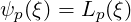
This filter is designed to output the energy spectrum of one-dimensional elements. It
transforms the solution field at each timestep into a orthogonal basis defined by the
functions
where Lp is the p-th Legendre polynomial. This can be used to show the presence of, for
example, oscillations in the underlying field due to numerical instability. The resulting output
is written into a file called session.eny by default. The following parameters are
supported:
| Option name | Required | Default | Description
|
OutputFile | ✗ | session | Prefix of the output filename
to which the energy spectrum
is written.
|
OutputFrequency | ✗ | 1 | Number of timesteps after
which output is written.
|
| |
An example syntax is given below:
1<FILTER TYPE="Energy1D">
2 <PARAM NAME="OutputFile">EnergyFile</PARAM>
3 <PARAM NAME="OutputFrequency">10</PARAM>
4</FILTER>
3.4.15 Reynolds stresses
Note: This filter is only supported for the incompressible Navier-Stokes solver.
This filter is an extended version of the time-average fields filter (see Section 3.4.16). It
outputs not only the time-average of the fields, but also the Reynolds stresses. The same
parameters supported in the time-average case can be used, for example:
1<FILTER TYPE="ReynoldsStresses">
2 <PARAM NAME="OutputFile">MyAverageField</PARAM>
3 <PARAM NAME="RestartFile">MyAverageRst.fld</PARAM>
4 <PARAM NAME="OutputFrequency">100</PARAM>
5 <PARAM NAME="SampleFrequency"> 10 </PARAM>
6</FILTER>
By default, this filter uses a simple average. Optionally, an exponential moving average can be
used, in which case the output contains the moving averages and the Reynolds stresses
calculated based on them. For example:
1<FILTER TYPE="ReynoldsStresses">
2 <PARAM NAME="OutputFile">MyAverageField</PARAM>
3 <PARAM NAME="MovingAverage">true</PARAM>
4 <PARAM NAME="OutputFrequency">100</PARAM>
5 <PARAM NAME="SampleFrequency"> 10 </PARAM>
6 <PARAM NAME="alpha"> 0.01 </PARAM>
7</FILTER>
3.4.16 Time-averaged fields
This filter computes time-averaged fields for each variable defined in the session file. Time
averages are computed by either taking a snapshot of the field every timestep, or alternatively
at a user-defined number of timesteps N. An output is produced at the end of the simulation
into session_avg.fld, or alternatively every M timesteps as defined by the user,
into a sequence of files session_*_avg.fld, where * is replaced by a counter. This
latter option can be useful to observe statistical convergence rates of the averaged
variables.
This filter is derived from FieldConvert filter, and therefore support all parameters available in
that case. The following additional parameter is supported:
| Option name | Required | Default | Description
|
SampleFrequency | ✗ | 1 | Number of timesteps at which
the average is calculated, N.
|
RestartFile | ✗ | | Restart file used as initial
average. If no extension is
provided, it is assumed as .fld
|
| |
As an example, consider:
1<FILTER TYPE="AverageFields">
2 <PARAM NAME="OutputFile">MyAverageField</PARAM>
3 <PARAM NAME="RestartFile">MyRestartAvg.fld</PARAM>
4 <PARAM NAME="OutputFrequency">100</PARAM>
5 <PARAM NAME="SampleFrequency"> 10 </PARAM>
6</FILTER>
This will create a file named MyAverageField.fld averaging the instantaneous
fields every 10 time steps. The averaged field is however only output every 100 time
steps.
3.4.17 ThresholdMax
The threshold value filter writes a field output containing a variable m, defined by the time at
which the selected variable first exceeds a specified threshold value. The default name of the
output file is the name of the session with the suffix _max.fld. Thresholding is applied based
on the first variable listed in the session by default.
The following parameters are supported:
| Option name | Required | Default | Description
|
OutputFile | ✗ | session_max.fld | Output filename to
which the threshold
times are written.
|
ThresholdVar | ✗ | first variable name | Specifies the variable
on which
the threshold will be
applied.
|
ThresholdValue | ✓ | - | Specifies the
threshold value.
|
InitialValue | ✓ | - | Specifies the initial
time.
|
StartTime | ✗ | 0.0 | Specifies the time
at which to start
recording.
|
| |
An example is given below:
1 <FILTER TYPE="ThresholdMax">
2 <PARAM NAME="OutputFile"> threshold_max.fld </PARAM>
3 <PARAM NAME="ThresholdVar"> u </PARAM>
4 <PARAM NAME="ThresholdValue"> 0.1 </PARAM>
5 <PARAM NAME="InitialValue"> 0.4 </PARAM>
6 </FILTER>
which produces a field file threshold_max.fld.
3.4.18 ThresholdMin value
Performs the same function as the ThresholdMax filter (see Section ??) but records the time
at which the threshold variable drops below a prescribed value.