Compressible flows can be characterised by abrupt changes in flow variables within the flow domain often referred to as shocks. These discontinuities can lead to numerical instabilities (Gibbs phenomena). This problem is prevented by locally adding a diffusion term to the equations to damp the numerical oscillations.
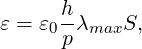
For the non-smooth artificial viscosity model the added artificial viscosity is constant in each element and discontinuous between the elements. The Euler system is augmented by an added Laplacian term on right hand side of equation 9.1 [36]. The diffusivity of the system is controlled by a variable viscosity coefficient ε. For consistency ε is proportional to the element size and inversely proportional to the polynomial order. Finally, from physical considerations ε needs to be proportional to the maximum characteristic speed of the problem. The final form of the artificial viscosity is
|
| (9.8) |
where S is a sensor.
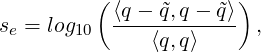
As shock sensor, a modal resolution-based indicator is used
 | (9.9) |
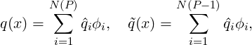
where ⟨⋅,⋅⟩ represents a L2 inner product, q and  are the full and truncated expansions of a
state variable (in our case density)
are the full and truncated expansions of a
state variable (in our case density)
 | (9.10) |
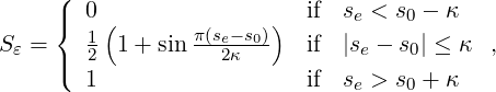
then the constant element-wise sensor is computed as follows
 | (9.11) |
where s0 = sκ - 4.25 log10(p).
To enable the non-smooth viscosity model, the following line has to be added to the
SOLVERINFO section:
The diffusivity and the sensor can be controlled by the following parameters:


A sensor based p-adaptive algorithm is implemented to optimise the computational cost and
accuracy. The DG scheme allows one to use different polynomial orders since the coupling
between different elements are determined by common numerical fluxes and there is no further
coupling between the elements. Furthermore, the initial p-adaptive algorithm uses the same
sensor as the shock capturing algorithm to identify the smoothness of the local
solution so it rather straightforward to implement both algorithms at the same
time.
The polynomial order in each element can be adjusted based on the sensor value that is
obtained. Initially, a converged solution is obtained after which the sensor in each element is
calculated. Based on the determined sensor value and the pre-defined sensor thresholds, it is
decided to increase, decrease or maintain the degree of the polynomial approximation in each
element and a new converged solution is obtained.
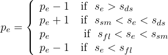 | (9.12) |
For now, the threshold values se, sds, ssm and sfl are determined empirically by looking at the sensor distribution in the domain. Once these values are set, two .txt files are outputted, one that has the composites called VariablePComposites.txt and one with the expansions called VariablePExpansions.txt. These values have to copied into a new .xml file to create the adapted mesh.
Aliasing effects, arising as a consequence of the nonlinearity of the underlying problem, need to be address to stabilise the simulations. Aliasing appears when nonlinear quantities are calculated at an insufficient number of quadrature points. We can identify two types of nonlinearities:
We consider two de-aliasing strategies based on the concept of consistent integration:
Since Nektar++ tackles separately the PDE and geometric aliasing during the projection and solution of the equations, to consistently integrate all the nonlinearities in the compressible NavierStokes equations, the quadrature points should be selected based on the maximum order of the nonlinearities:
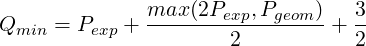 | (9.13) |
where Qmin is the minimum required number of quadrature points to exactly integrate the highest-degree of nonlinearity, Pexp being the order of the polynomial expansion and Pgeom being the geometric order of the mesh. Bear in mind that we are using a discontinuous discretisation, meaning that aliasing effect are not fully controlled, since the boundary terms introduce non-polynomial functions into the problem.
To enable the global de-aliasing technique, modify the number of quadrature points by:
where NUMMODES corresponds to P+1, where P is the order of the polynomial used to
approximate the solution. NUMPOINTS specifies the number of quadrature points.
In this example, we solve a compressible flow past a circular cylinder using an implicit
discontinuous Galerkin compressible flow solver as shown in figure 9.2. For the implicit
time-integration schemes, TimeStep or CFL can be adopted to control the time step. For the
case of using CFL, the CFL number can grow from CFL to CFLEnd by a ratio of CFLGrowth to
adjust the time step at different stages of the simulation.
The CFL number, growing CFL number and the maximum value of the CFL number are controlled by the following parameters as also described in section 9.3
In this case, the numerical simulation starts from a CFL number of 0.1 and grows by a ratio of
1.1 up to a maximum value of CFL number of 2.0. Note that the CFLEnd parameter may
assume higher values, depending on the strategy adopted. In addition, there is no need to
define the TimeStep parameter, since the time step size is calculated based on the CFL
number in each time step.
Since we are solving an implicit time-integration scheme, we must specify to the solver
information the EQType which corresponds to an implicit solver. It should be noted that
currently the CFS solver only supports NavierStokesImplicitCFE and EulerImplicitCFE.
There are some other parameters controlling the performance of the implicit solver.
NonlinIterTolRelativeL2 determines the convergence tolerance of the nonlinear system
solver relative to the initial nonlinear system residual. NekNonlinSysMaxIterations is the
maximum iteration number of the nonlinear system solver. LinSysRelativeTolInNonlin
determines the convergence tolerance of linear system solver in each nonlinear iteration.
NekLinSysMaxIterations is the maximum iteration number of the linear system solver in
each nonlinear iteration. LinSysMaxStorage determines the maximum number of variable
vector allowed to store in the linear system solver. Specifically for GMRES solver, the GMRES
solver will be restarted if NekLinSysMaxIterations is larger than LinSysMaxStorage and
thus LinSysMaxStorage determines the storage consumption of the GMRES solver. Regarding
the parameters to control the preconditioners in GMRES, PreconMatFreezNumb specifies
the number of time steps to freeze the preconditioning matrices, in other words,
the preconditioning matrices will be updated based on the number of time steps
provided by the user. PreconItsStep determines the number of preconditioning
iterations to calculate the preconditioned vector. The default parameters are listed
below.
Here, we choose to solve the compressible Navier-Stokes equations and use the 2nd order Singly Diagonally Implicit Runge–Kutta (SDIRK) method.