11.9 Imposing a constant flowrate

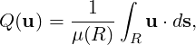
In some simulations, it may be desirable to drive the flow by fixing a value of the volumetric flux through a boundary surface. A common use case for this is a channel flow, where the inflow and outflow are treated using periodic boundary conditions, requiring a use of either a body force or a flowrate condition to drive the flow. Often, the use of a body force is sufficient, but in some cases (e.g. transitional or turbulent simulations), it may be difficult to determine the correct body force to use in order to attain a specific Reynolds number. The incompressible solver supports the use of an alternative forcing whereby the volumetric flux,

through a user-defined surface R of area μ(R) is kept constant. This is supported for standard two- and three-dimensional simulations, where R is a boundary region, as well as three-dimensional homogeneous simulations. In the latter case, the forcing can be imposed either in the homogeneous direction (in the x - y plane) or perpendicular to it (in the z direction).

The flowrate correction works by taking each timestep’s velocity field uⁿ, and computing a scalar α so that the corrected flow

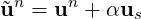
has the desired flowrate. Here, u_s is a linear Stokes solution that is calculated once at the start of the simulation, so that the condition is not expensive to implement.

To enable flowrate corrections, three things must be defined in the session file:

• The Flowrate parameter in the parameters section, which defines the desired value of the volumetric flux Q(u) through the reference region. To set a flux per unit surface of Q = 1 we would therefore define:
  1<PARAMETERS> 
  2  <P> Flowrate = 1.0 </P> 
  3</PARAMETERS>
• A boundary condition must be tagged with the Flowrate user-defined type to define the reference region R. For example, a 2D channel flow with periodic boundary conditions might use the following arrangement:
  1<BOUNDARYCONDITIONS> 
  2  <REGION REF="0"> 
  3    <P VAR="u" VALUE="[1]" USERDEFINEDTYPE="Flowrate" /> 
  4    <P VAR="v" VALUE="[1]" /> 
  5    <P VAR="p" VALUE="[1]" /> 
  6  </REGION> 
  7  <REGION REF="1"> 
  8    <P VAR="u" VALUE="[0]" /> 
  9    <P VAR="v" VALUE="[0]" /> 
  10    <P VAR="p" VALUE="[0]" /> 
  11  </REGION> 
  12</BOUNDARYCONDITIONS>
• a FlowrateForce function with components ForceX, ForceY and ForceZ that defines the direction in which the forcing will be applied. This should be a unit vector (i.e. of magnitude 1) and constant (i.e. not dependent on x, y, z or t). As an example, to impose a force in the x-direction we specify:
  1<FUNCTION NAME="FlowrateForce"> 
  2  <E VAR="ForceX" VALUE="1.0" /> 
  3  <E VAR="ForceY" VALUE="0.0" /> 
  4  <E VAR="ForceZ" VALUE="0.0" /> 
  5</FUNCTION>

Importantly, note that in homogeneous simulations where the forcing is in the z-direction only the Flowrate parameter should be specified, and the reference area R is taken to be the homogeneous plane.

Optionally, the IO_FlowSteps parameter can be defined. If set to a non-zero integer, this produces a file session.prs which records the value of α used in the flowrate correction, every IO_FlowSteps steps.