12.4 Examples

12.4.1 L-shaped domain

The first example is the classic L-shaped domain, in which an exact solution is known, which makes it an ideal test case [24]. The domain is the polygon formed from the vertices

The exact solution for the displacements is known in polar co-ordinates (r,θ) as

ur(r,θ)	=
uθ(r,θ)	=

where α ≈ 0.544483737… is the solution of the equation α sin(2ω) + sin(2ωα) = 0,

with λ and μ being the Lamé constants and ω = 3π∕4. Boundary conditions are set to be the exact solution and f = 0. The solution has a singularity at the origin, and so in order to test convergence h-refinement is required.

A simple example of how the linear elastic solver can be set up can be found in the Tests/L-shaped.xml session file in the linear elastic solver directory. A more refined domain with the obtained u solution is shown in figure 12.1. The solver can be run using the command:

LinearElasticSolver L-domain.xml

The obtained solution L-domain.fld can be applied to the mesh to obtain a deformed XML file using the deform module in FieldConvert:

FieldConvert -m deform L-domain.xml L-domain.fld L-domain-deformed.xml

12.4.2 Boundary layer deformation

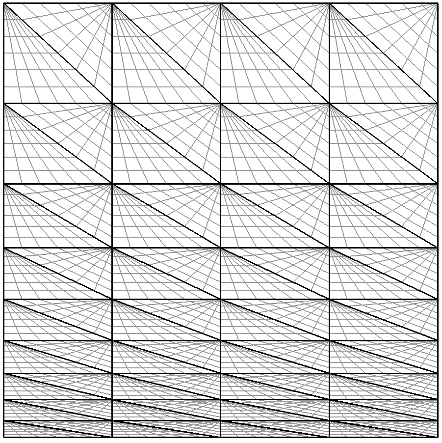
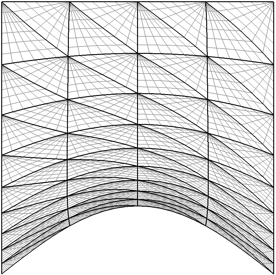
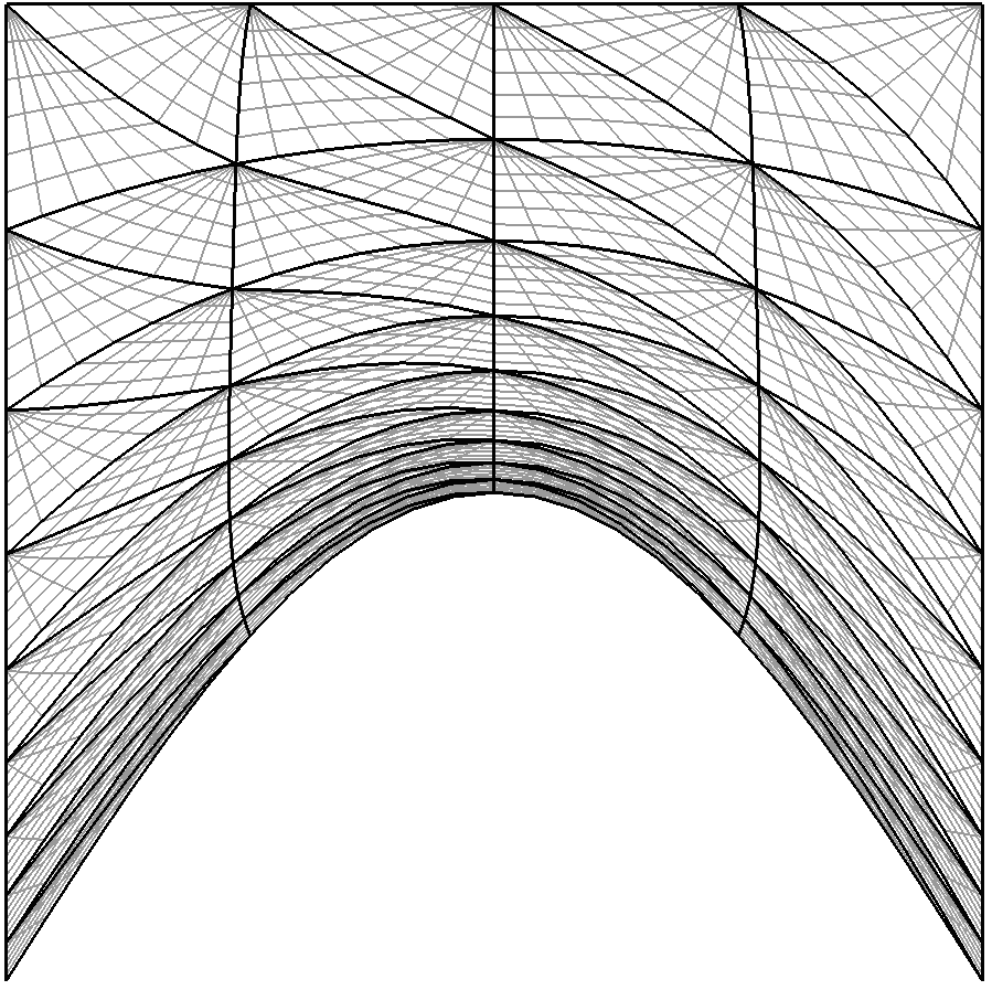
In this example we use the iterative elastic system to apply a large deformation to a triangular boundary layer mesh of a square mesh Ω = [0,1]². At the bottom edge, we apply a Dirichlet condition g = sin(πx) that is enforced by splitting it into N substeps, so that at each step we solve the system with the boundary condition gⁿ(x) = g(x)∕N. The process is depicted in figure 12.2.

The setup is very straightforward. The geometry can be found inside the file Examples/bl-mesh.xml and the conditions inside Examples/bl-conditions.xml. The solver can be set up using the following parameters, with NumSteps denoting N:

1  <SOLVERINFO> 
2    <I PROPERTY="EQTYPE" VALUE="IterativeElasticSystem" /> 
3  </SOLVERINFO> 
4 
5  <PARAMETERS> 
6    <P> nu       = 0.3 </P> 
7    <P> E        = 1.0 </P> 
8    <P> NumSteps = 100 </P> 
9  </PARAMETERS>

To identify the boundary that we intend to split up into substeps, we must assign the WALL tag to our boundary regions:

1  <BOUNDARYCONDITIONS> 
2    <REGION REF="0"> 
3      <D VAR="u" VALUE="0" USERDEFINEDTYPE="Wall" /> 
4      <D VAR="v" VALUE="0.5*sin(PI*x)" USERDEFINEDTYPE="Wall" /> 
5    </REGION> 
6    <REGION REF="1"> 
7      <D VAR="u" VALUE="0" /> 
8      <D VAR="v" VALUE="0" /> 
9    </REGION> 
10  </BOUNDARYCONDITIONS>

The solver can then be run using the command:

LinearElasticSolver bl-mesh.xml bl-conditions.xml

This will produce a series of meshes bl-mesh-%d.xml, where %d is an integer running between 0 and 100. If at any point the mesh becomes invalid, that is, a negative Jacobian is detected, execution will cease.