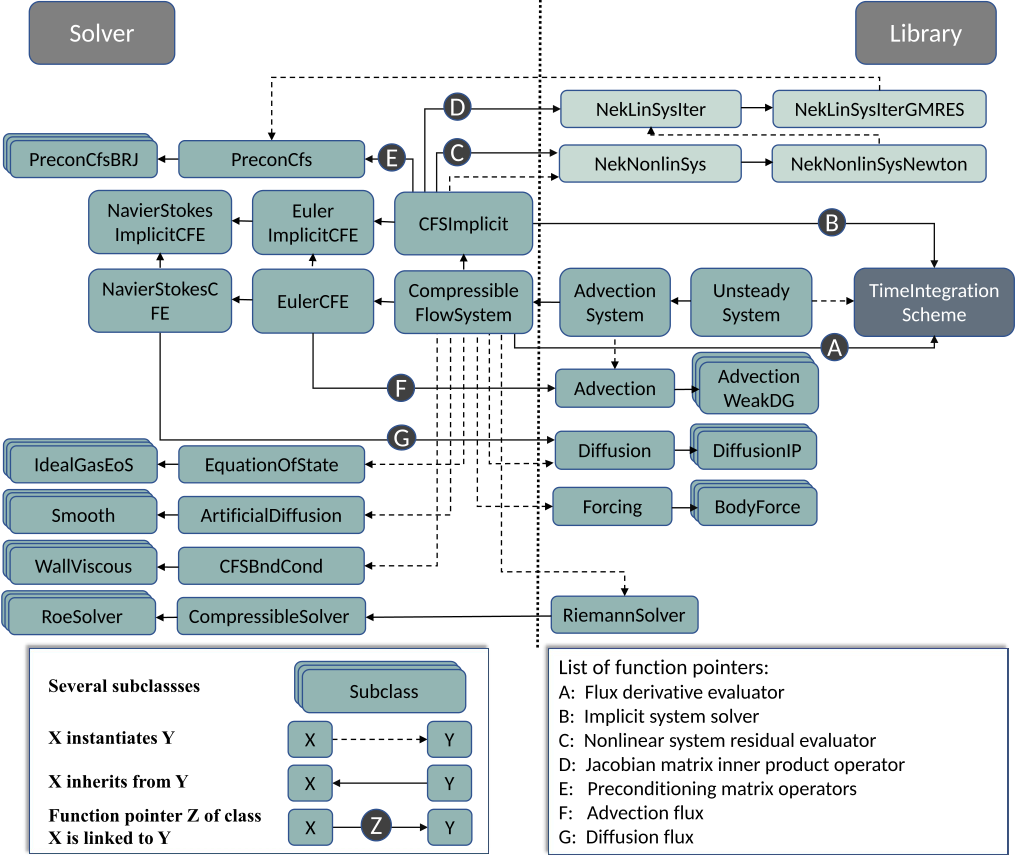
Figure 15.2 Class structure of the explicit and implicit solvers. The equation system classes
(
EulerCFE or NavierStokesCFE) contain access to the main functionalities of the solver,
such as time integration, and the solution fields. They make use of numerical methods from
the libraries, such as AdvectionWeakDG, and equations system related functions, such as the
advection flux ( F) and diffusion flux ( G), to form the spatial discretization operator A. The
spatial operator A and the time integration method form the explicit solver using the method of
lines. For the implicit solver, additional classes like the Newton solver ( NekNonlinSysNewton),
GMRES solver ( NekLinSysIterGMRES) and linear algebra solver of preconditioners (e.g.
PrecondCfsBRJ) are instantiated. Together with operators related to the nonlinear system ( C),
the Jacobian matrix ( D) and preconditioning matrix ( E), an implicit system solver ( B) is
constructed, which is linked to the implicit time integration scheme to form the implicit solver. is linked to the
time integration class using the pointer-to-function
is linked to the
time integration class using the pointer-to-function  ,M
,M
 ,J
,J  j =
j =  -1
-1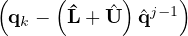
 J
J